Buying high-quality stocks and avoiding low-quality ones can improve investment returns. In this post, I use Alphalens and Zipline to analyze the Piotroski F-Score, a composite measure of a firm's financial health and quality.

What is the Piotroski F-Score?

Joseph Piotroski, an accounting professor, developed the Piotroski F-Score in 2000 as a way to identify high-quality stocks. The Piotroski F-Score is often used by value investors to avoid the so-called value trap, that is, the trap of buying cheap stocks that are only cheap because they are in trouble. (This is how Piotroski used the F-Score in the original paper.) However, the F-Score can also be used as a standalone factor and is commonly referred to as the quality factor (although some practitioners define quality using alternative formulas).

The Piotroski F-Score is a composite factor comprising multiple sub-factors. It is calculated as the sum of 9 true/false criteria, resulting in a possible score of 0-9. Points are awarded as follows:

• Profitability Criteria:
  • 1 point if return on assets (ROA) is positive in the current year
  • 1 point if operating cash flow is positive in the current year
  • 1 point if ROA is higher in the current period than in the previous year
  • 1 point if cash flow from operations is higher than ROA (quality of earnings)
• Funding Criteria:
  • 1 point if long term debt is lower in the current period than in the previous year (decreased leverage)
  • 1 point if current ratio is higher in the current period than in the previous year (more liquidity)
  • 1 point if no new shares were issued in the last year (lack of dilution)
• Operating Efficiency Criteria:
  • 1 point if gross margin is higher in the current period than in the previous year
  • 1 point if asset turnover ratio is higher in the current period than in the previous year

The three broad categories of the Piotroski F-Score criteria (profitability criteria, funding criteria, and operating efficiency criteria) correspond roughly to the themes previously explored in this series. We saw that profitability is good (see: Analyzing the Profitability Factor with Alphalens), too much debt is bad (see: Financial Distress Factors: the Altman Z-Score and Interest Coverage Ratio), and improving operating efficiency is good (see: What's Better, High Profit Margins or Improving Profit Margins?). The Piotroski F-Score combines multiple independently useful factors into a single score.

The Piostroski F-Score in Pipeline

Using the Piotroski F-Score in Pipeline is simple, as a built-in factor is provided:

from zipline.pipeline import sharadar

f_score = sharadar.PiotroskiFScore()

However, to demonstrate how multi-factor scores can be constructed using any criteria the researcher wants, let's peek at a snippet of the source code to see how the score is computed. First, we compute the individual boolean criteria (e.g. return_on_assets > 0), then we call as_factor() to convert the boolean output to 1s or 0s. The resulting numbers are then summed to produce the final F-Score:

...
# ART = as reported, trailing 12 months fundamentals
fundamentals = sharadar.Fundamentals.slice('ART')

# get necessary fields
return_on_assets = fundamentals.ROA.latest
operating_cash_flow = fundamentals.NCFO.latest
...

# compute score
f_scores = (
    (return_on_assets > 0).as_factor()
    + (operating_cash_flow > 0).as_factor()
    ...
)

Alphalens Analysis of the Piotroski F-Score

I use Alphalens to analyze how the Piotroski F-Score impacts stock performance. I group stocks into 3 buckets based on their F-Scores: a bucket for stocks with low scores (0-3), another bucket for medium scores (4-6), and a third bucket for high scores (7-9). I include market cap as a grouping factor to see if the F-Score's predictive efficacy differs for small caps vs large caps.

from zipline.pipeline import Pipeline, sharadar
import alphalens as al

fundamentals = sharadar.Fundamentals.slice("ART")
marketcap = fundamentals.MARKETCAP.latest

f_scores = sharadar.PiotroskiFScore()

pipeline = Pipeline(
    columns={
        "quality": f_scores,
        "size": marketcap.quantiles(4)
    }
)

al.from_pipeline(
    pipeline,
    start_date="1999-02-01",
    end_date="2023-06-30",
    periods=[1, 5, 21],
    factor="quality",
    # 3 bins: 0-3, 4-6, 7-9
    bins=[-1,3,6,9],
    groupby=[
        "size",
    ],
    segment="Y",
)

Results

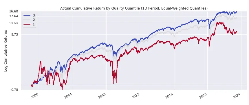
30% of stocks have low F-Scores (0-3), 55% have medium F-Scores (4-6), and 15% have high F-Scores (7-9). The following plot shows the cumulative return of each basket of stocks. The high-quality stocks (blue line) handily outperform the low-quality stocks (red line), largely as a result of experiencing smaller drawdowns during bear markets (including the most recent bear market in 2022):

Market Cap Subgroup Analysis

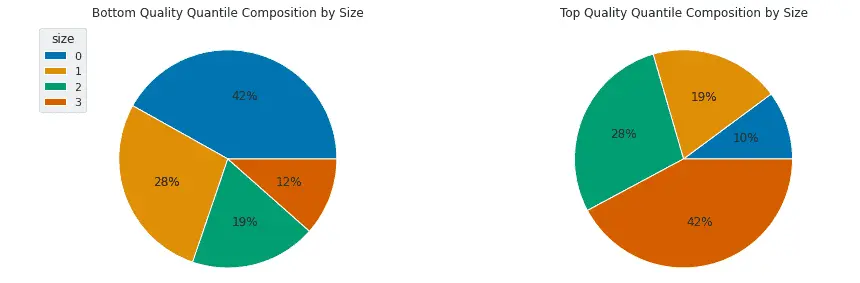
Next I look at the composition of the low- and high-quality buckets by market cap. The low-quality bucket (left-hand pie plot) is dominated by stocks in the smallest two quartiles (quartiles 0 and 1, shaded blue and light orange), while the high-quality bucket (right-hand pie plot) is dominated by stocks in the largest two quartiles (quartiles 2 and 3, shaded green and dark orange). The finding that low-quality stocks tend to be small caps while high-quality stocks tend to be large caps is intuitive: all companies start out small, and the higher-quality ones grow to become large companies while the lower-quality ones remain small.

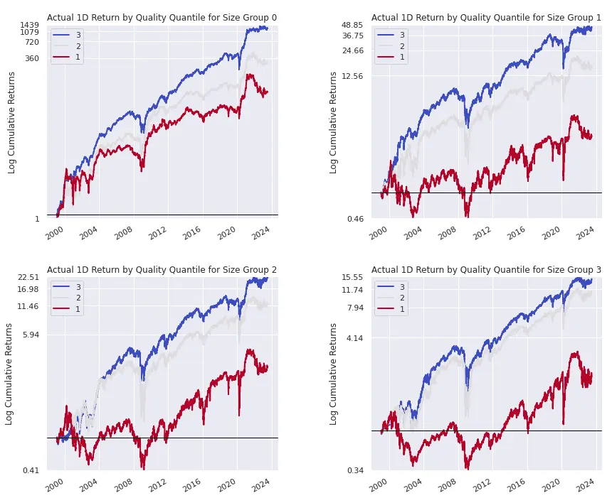
The next plot shows the cumulative return by F-Score bucket for each of the 4 market cap quartiles, where quartile 0 contains the smallest companies and quartile 3 contains the largest. Appealingly, the performance spread between high- and low-quality stocks is not limited to small cap stocks (quartile 0) but is robust among all quartiles, including large companies (quartile 3). This means that investors can adopt the quality factor in their investing strategies without having to deal with the challenges of trading small caps:

Should we apply a value filter to a high-quality screen?

Unlike valuation metrics such as the price-to-earnings ratio or enterprise multiple, the Piotroski F-Score does not take into account a stock's current market price. A portfolio of high-quality stocks may include stocks that are expensive or cheap by valuation measures.

As mentioned above, Joseph Piotroski originally proposed the F-Score as a quality filter to be applied on top of a value screen. That is, an investor would select a basket of cheap stocks, then apply the F-Score to weed out the low-quality stocks within that subset.

In the following analysis, I proceed in the opposite order, applying value as a filter on top of a high-quality screen. To do so, I create a new pipeline that limits the analysis to high-quality stocks (F-Score >= 7). Since the Piotroski F-Score works not only on small caps but on large caps, I also choose to limit the analysis to the top 50% of stocks by market cap. Within this universe of high-quality, large-cap stocks, I divide stocks into 4 buckets by their valuation (using enterprise multiple as my valuation ratio) and use Alphalens to see if cheap high-quality stocks outperform expensive high-quality stocks. The modified code looks like this:

enterprise_multiple = fundamentals.EVEBITDA.latest

are_high_quality = f_scores >= 7
are_large_caps = marketcap.percentile_between(50, 100)

screen = are_high_quality & are_large_caps

pipeline = Pipeline(
    columns={
        "value": enterprise_multiple,
    },
    screen=screen
)

al.from_pipeline(
    pipeline,
    start_date="1999-02-01",
    end_date="2023-06-30",
    periods=[1, 5, 21],
    factor="value",
    quantiles=4,
    segment="Y",
)

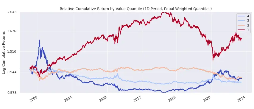
To highlight the spread between quartiles, the following plot shows the relative cumulative return (not actual cumulative return) of each value quartile. The cheapest high-quality stocks are represented by quartile 1 (red line), while the most expensive (but still high quality) stocks are represented by quartile 4 (blue line). Cheap, high-quality stocks significantly outperformed other high-quality stocks from around 2000 to 2015, but then the relationship reversed from 2015 to early 2020. Since 2020, cheap, high-quality stocks have resumed outperforming:

Zipline Trading Strategy: High-Quality S&P 500 Stocks

A typical research workflow with Pipeline is to use Alphalens to learn how a factor behaves in different areas of the market, then use Zipline to apply the insights to a particular trading strategy. With Alphalens, we ignore the practical constraints of trading (e.g. liquidity, transaction costs, and preferred number of holdings) and focus on the factor's performance. Once we know where alpha can be found, we use Zipline to craft a trading strategy that is practical to implement and deploy.

Along these lines, I use Zipline to backtest a simple trading strategy based on my Alphalens research. The strategy focuses on large-cap, high-quality stocks, purchasing an equal-weighted portfolio of S&P 500 stocks with F-Scores >= 7 and rebalancing monthly. The strategy code is simple enough to paste in its entirety:

import zipline.api as algo
from zipline.pipeline import Pipeline, sharadar
from zipline.finance import commission

def initialize(context: algo.Context):

    algo.set_benchmark(algo.symbol('SPY'))
    algo.set_commission(commission.PerShare(0.005))

    # select S&P500 stocks with F Scores >= 7
    screen = sharadar.SP500.in_sp500.latest
    f_scores = sharadar.PiotroskiFScore()
    screen &= f_scores >= 7

    pipe = Pipeline(screen=screen)
    algo.attach_pipeline(pipe, 'pipe')

    # rebalance monthly
    algo.schedule_function(
        rebalance,
        date_rule=algo.date_rules.month_start())

def rebalance(context: algo.Context, data: algo.BarData):

    desired_portfolio = algo.pipeline_output('pipe').index

    current_positions = context.portfolio.positions

    # open new positions and rebalance existing positions
    for asset in desired_portfolio:
        algo.order_target_percent(asset, 1 / len(desired_portfolio))

    # liquidate positions that no longer pass the screen
    for asset in current_positions:
        if asset not in desired_portfolio:
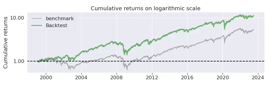
            algo.order_target_percent(asset, 0)

The cumulative performance of the strategy vs the benchmark, SPY, is shown below:

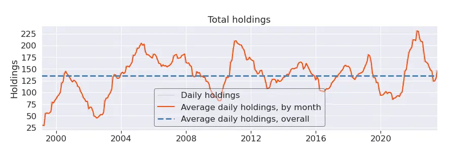
The following plot shows that the total number of holdings generally varies between 100 and 200. Depending on the trader's preferences, a possible next step might be to refine the strategy to reduce the number of holdings. One way to do this, in line with the above research, would be to buy only the cheapest high-quality stocks, rather than buying all high-quality stocks as was done here.

Explore this research on your own

This research was created with QuantRocket. Clone the fundamental-factors repository to get the code and perform your own analysis.