Exploratory Data Analysis of Fundamental Factors
Wed Jun 14 2023 by Brian StanleyWhen researching fundamental factors, analyzing alpha shouldn't be your first step. You can save time and spot issues early by starting with a basic exploration of your factor's distribution and statistical properties, a process known as exploratory data analysis (EDA). This post looks at operating margin, a profitability ratio, to demonstrate what you can learn from exploratory data analysis.
Why EDA is Worthwhile
Exploratory data analysis is an often overlooked step in the research process. While gaining a basic understanding of a factor's statistical characteristics might not seem as interesting as plotting the factor performance with Alphalens or running a backtest, investing a little time upfront to get to know your data can save you significant time and confusion later by highlighting ways that you must massage the data or tweak your computations to achieve the desired results.
If there's an issue with your factor and you skip EDA, two types of problems can emerge. First, the issue may manifest later in your analysis, at which point you will be farther downstream from the source of the issue, making it harder to trace. Second, and worse, the problem might never become apparent at all, instead leading to incorrect results that cause you to misinterpret the data.
What is Operating Margin?
Operating margin is a profitability ratio that measures how much profit a company makes on each dollar of sales after paying operating costs such as wages, rent, and utilities. Operating margin is one of three main profitability ratios, along with gross margin and net margin. The three ratios are distinguished by what they subtract from revenue, with gross margin, operating margin, and net margin subtracting increasingly more from revenue:
- Gross margin subtracts the cost of goods sold (COGS) from revenue
- Operating margin additionally subtracts operating expenses, which includes wages, overhead, and depreciation
- Net margin additionally subtracts all other expenses, including taxes, interest, and extraordinary items
Arguably, operating margin is the "Goldilocks" ratio for understanding a company's core performance, as gross margin doesn't subtract enough from revenue while net margin subtracts too much. Gross margin only subtracts the cost of goods sold, but a business has many other intrinsic costs, such as paying its employees. On the other hand, net margin subtracts expenses that are extrinsic to a company's core performance and often temporary, such as extraordinary items and interest costs.
How to Calculate Operating Margin in Pipeline
Let's dive into the data. We can calculate operating margin in Pipeline by dividing operating income (OPINC) by revenue:
from zipline.pipeline import sharadar

# ART = as-reported, trailing-twelve-month fundamentals
fundamentals = sharadar.Fundamentals.slice('ART')
operating_margin = fundamentals.OPINC.latest / fundamentals.REVENUE.latest
Let's look at a year of operating margin data. At this exploratory stage, a year of data or even less will suffice since the purpose is simply to get a basic understanding of the data distribution and characteristics. We can run the pipeline and get a DataFrame of results as follows:
from zipline.pipeline import Pipeline
from zipline.research import run_pipeline

pipeline = Pipeline(
    columns={
        'operating_margin': operating_margin,
    }
)
results = run_pipeline(pipeline, '2022-01-01', '2022-12-31')
Start with pandas describe()
An easy and fail-safe first way to explore the data is using pandas's describe() method, which computes summary statistics for each column in the DataFrame. We will visualize the data distribution with a histogram later, but describe() is nice because it works for any kind of data and doesn't require us to think in advance about what kind of plot is best suited to the data, a task that can be tricky when we don't yet have a basic understanding of the data distribution.
results.describe()| operating_margin | |
|---|---|
| count | 1.036630e+06 |
| mean | NaN |
| std | NaN |
| min | -inf |
| 25% | -2.471616e-01 |
| 50% | 6.503638e-02 |
| 75% | 2.044458e-01 |
| max | inf |
Oops, Division by Zero
We immediately notice the NaN and inf values in the describe() output above. What's going on here? Oops, we are dividing operating income by revenue, and revenue can be 0 (companies with no sales). Dividing by zero causes pandas/numpy to compute +/-infinity for max and min, and the inf values cause the NaN values for mean and standard deviation. A quick check of describe() has highlighted a problem that we should correct before going any further.
We can re-write the operating margin factor to ignore companies with no revenue as follows:
revenue = fundamentals.REVENUE.latest
operating_margin = fundamentals.OPINC.latest / revenue.where(revenue > 0)
Re-running the pipeline and describe() method, the NaN and inf values are gone:
| operating_margin | |
|---|---|
| count | 944237.000000 |
| mean | -40.714307 |
| std | 4989.082683 |
| min | -841260.400000 |
| 25% | -0.065883 |
| 50% | 0.081923 |
| 75% | 0.222380 |
| max | 7.001749 |
A Reminder that Operating Margin Can Be Negative
What else can we learn from the describe() output? Intuitively, we can think of profit margin as the amount of revenue left over after paying expenses. A company with no revenue left over after expenses would have a profit margin of 0, while a company with no expenses would have a profit margin of 1.
But the describe() output reminds us that operating margin is not bounded by 0 and 1. First of all, operating income can be negative, so operating margin can also be negative: a company can spend arbitrarily more than it brings in as revenue. (The minimum operating margin in our sample is a disastrous -84 million percent.) If you were approaching the data with the idea of researching profitable companies, describe() would provide a useful reminder that there are also many unprofitable companies in the stock market. Depending on your goals, you may want to include the unprofitable companies in your analysis or exclude them.
Operating Margin Greater than 100%?
A second revelation of describe() is more puzzling: operating margin can be greater than 1. (The maximum in our sample is approximately 7, that is, 700%.) This violates the intuitive understanding of profit margin as the amount of revenue left over after paying expenses. How can there be more than 100% of revenue left over after paying expenses?
To see what's going on, we need to look at some specific examples. We'll re-run the pipeline, but this time we'll screen for stocks with operating margin greater than 1, and we will include in the output all of the relevant columns from which operating margin is derived (which we can look up via the column definitions for OPINC and REVENUE). This will help us see where the unexpected result is coming from.
pipeline = Pipeline(
    columns={
        'operating_margin': operating_margin, # operating_margin = OPINC / REVENUE
        'revenue': fundamentals.REVENUE.latest,
        'operating_income': fundamentals.OPINC.latest, # OPINC = GP - OPEX
        'gross_profit': fundamentals.GP.latest, # GP = REVENUE - COR
        'cost_of_revenue': fundamentals.COR.latest,
        'operating_expenses': fundamentals.OPEX.latest
    },
    screen=operating_margin > 1
)

results = run_pipeline(pipeline, '2022-01-01', '2022-12-31')
results.sort_values('operating_margin', ascending=False).drop_duplicates().head(2)| operating_margin | revenue | operating_income | gross_profit | cost_of_revenue | operating_expenses | ||
|---|---|---|---|---|---|---|---|
| date | asset | ||||||
| 2023-01-03 | STRS | 7.001749 | 10866000.0 | 76081000.0 | 8507000.0 | 2359000.0 | -67574000.0 |
| 2022-12-19 | AMBC | 1.517751 | 338000000.0 | 513000000.0 | 694000000.0 | -356000000.0 | 181000000.0 |
In the output, we spot the issues (highlighted in red): operating expenses in one case, and cost of revenue in another, are negative, which accounts for operating margin being greater than 1. A negative operating expense or cost of revenue is unexpected and may indicate an unusual one-time accounting adjustment made by the company; further investigation (such as viewing the full report on the SEC website) would be required to determine with certainty. Regardless, for the purpose of our profitability analysis, we probably don't want to treat a company with negative operating expenses or negative cost of revenue as though it were extraordinarily profitable. Therefore, we can refine our profitability factor further by excluding these companies.
# exclude companies with negative operating expenses or negative cost of revenue
opex = fundamentals.OPEX.latest
cor = fundamentals.COR.latest
operating_margin = operating_margin.where((opex > 0) & (cor > 0))
After re-running the refined pipeline, the output from describe() conforms better to expectations, as the maximum operating margin is now slightly below 1:
| operating_margin | |
|---|---|
| count | 777637.000000 |
| mean | -40.002138 |
| std | 5480.989899 |
| min | -841260.400000 |
| 25% | -0.064361 |
| 50% | 0.067519 |
| 75% | 0.165043 |
| max | 0.965168 |
Visualizing the Data Distribution
Now that we've refined our factor to exclude unusual cases, let's look at a histogram of operating margin to get a better feel for its distribution. We can use pandas's plot.hist() method to do so, which is appealingly simple. However, the plot we get for the data on the first try is not very informative, as there is only a single bar:
results.plot.hist()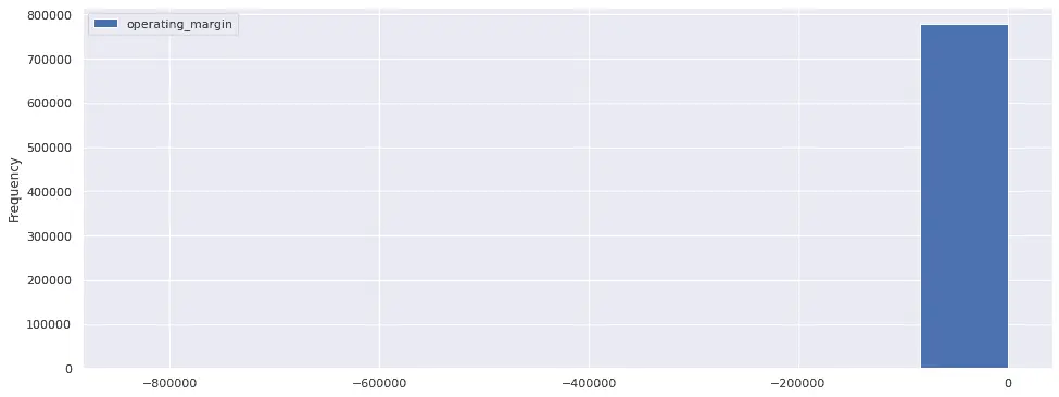
What's going on? Notice the extreme negative values on the X axis. This is a hint that negative outliers (companies with extremely negative operating margins) are causing most values to be crammed in a single bin. We can fix this by using the range argument to hist() to zoom in on the bulk of the distribution. In addition, we'll increase the number of bins to 20, from the default 10. Now the histogram looks sensible:
results.plot.hist(bins=20, range=(-1, 1))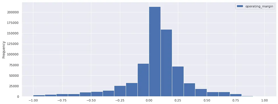
Clipping Outliers
Using range to zoom in on the distribution is useful for viewing the histogram, but it doesn't remove the outliers from the pipeline output itself. To facilitate using the pipeline output in Alphalens or Zipline, perhaps it would be a good idea to deal with the outliers directly in Pipeline. Beyond a certain point, increasingly negative operating margins don't provide useful additional information; it's enough to know that the company is very unprofitable.
A reasonable solution is to clip the values to -1, meaning that any values less than -1 will be replaced with -1:
operating_margin = operating_margin.clip(min_bound=-1, max_bound=1)After re-running the pipeline with the clipped factor, we can plot the histogram without using range:
results.plot.hist(bins=20)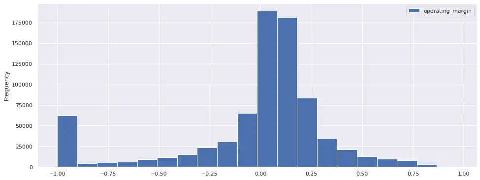
Notice that, unlike the previous histogram which ignored data outside the (-1, 1) range, in this histogram the clipped values cluster at -1. In other words, the previous histogram included a subset of the data, while this histogram includes all the data.
Conclusion
While exploratory data analysis is arguably not the most exciting step of the research process since it doesn't tell us a factor's predictive value, it is an important preparatory step that helps ensure that subsequent research is meaningful. Our EDA of the operating margin factor has helped us deal with several issues that might have caused problems later, such as companies with no revenue, companies with negative operating expenses, and extreme negative outliers. We've established a good foundation to explore the factor's predictive value with Alphalens in a subsequent post.
Explore this research on your own
This research was created with QuantRocket. Clone the fundamental-factors repository to get the code and perform your own analysis.
quantrocket codeload clone 'fundamental-factors' Send a Message