Intraday trading strategies offer great promise as well as great peril. This post explores an intraday trading strategy for crude oil calendar spreads and highlights the impact of transaction costs on its profitability.

Background

In a previous post, I explored an end-of-day pairs trading strategy in which the chief difficulty was to find suitable pairs. Pairs that cointegrate in-sample often cease to cointegrate out-of-sample.

Futures calendar spreads present an intriguing alternative to equity pairs because futures contracts for the same underlying are closely related to each other and thus seem unlikely to wander apart. The roll returns of futures can cause divergence between individual contracts over time, but this is unlikely to be a significant factor at an intraday time frame.

The mechanics of trading calendar spreads

To backtest an intraday calendar spread strategy for crude oil futures (symbol CL), I first collect 1-minute bid/ask bars for all CL futures contracts from Interactive Brokers.

After loading the prices into a pandas DataFrame, I use the function get_contract_nums_reindexed_like to obtain a DataFrame showing each contract's numerical sequence in the contract chain as of any given date:

>>> from quantrocket.master import get_contract_nums_reindexed_like
>>> contract_nums = get_contract_nums_reindexed_like(bids, limit=3)
>>> contract_nums.head()
ConId            CLM9       CLZ9       CLK9       CLJ9       CLN9
Date
2019-03-04        3.0        NaN        2.0        1.0        NaN
2019-03-05        3.0        NaN        2.0        1.0        NaN
2019-03-06        3.0        NaN        2.0        1.0        NaN
2019-03-07        2.0        NaN        1.0        NaN        3.0
2019-03-08        2.0        NaN        1.0        NaN        3.0
2019-03-11        2.0        NaN        1.0        NaN        3.0

I isolate the bids and asks for contract months 1 and 2 by masking the prices with the respective contract nums and taking the mean of each row. In taking the mean, I rely on the fact that the mask leaves only one non-null observation per row, thus the mean simply gives us that observation.

are_month_1_contracts = contacts_nums == 1
month_1_bids = bids.where(are_month_1_contracts).mean(axis=1)
month_1_asks = asks.where(are_month_1_contracts).mean(axis=1)

are_month_2_contracts = contacts_nums == 2
month_2_bids = bids.where(are_month_2_contracts).mean(axis=1)
month_2_asks = asks.where(are_month_2_contracts).mean(axis=1)

I then use the bids and asks to compute the calendar spread. To reflect the fact that I must buy at the ask and sell at the bid, I compute the spread differently for the purpose of identifying long vs short opportunities:

# Buying the spread means buying the month 1 contract at the ask and
# selling the month 2 contract at the bid
spreads_for_buys = month_1_asks - month_2_bids

...

# Selling the spread means selling the month 1 contract at the bid
# and buying the month 2 contract at the ask
spreads_for_sells = month_1_bids - month_2_asks

I use the spreads to construct Bollinger Bands set two standard deviations away from the spread's 60-minute moving average, and I buy (sell) the spread when it moves below (above) its lower (upper) band.

The Impact of Transaction Costs

First, using contract months 1 and 2, I backtest the intraday calendar spread strategy without transaction costs. That is, I apply no commissions, and I assume fills at the bid-ask midpoint. The backtest shows an attractive equity curve with a CAGR of 9% and a Sharpe ratio of 2.58. Evidently CL contracts reliably re-converge after divergences.

Next, I apply commissions, and I model buying at the ask and selling at the bid using the following code:

are_buys = positions.diff() > 0
are_sells = positions.diff() < 0
midpoints = (bids + asks) / 2
trade_prices = asks.where(are_buys).fillna(bids.where(are_sells)).fillna(midpoints)

With transaction costs, the CAGR is -91% and the Sharpe ratio is -21. The strategy's daily turnover is around 7,000%, indicating approximately 35 round-trip trades per day. The transaction costs from so much trading swamp the strategy's gross profit.

Ideas to Reduce Transaction Costs

Since the calendar spread strategy is profitable before transaction costs but unprofitable after costs, a natural next step is to search for special circumstances in which the profitability survives the transaction costs. Is it possible to make the strategy be more selective and trade less frequently? Below are several possible avenues to explore.

Use more distant calendar months

I opted to create spreads using contract months 1 and 2, but there are many other contracts available. The following heat maps shows the average dollar spread between different CL contract months:

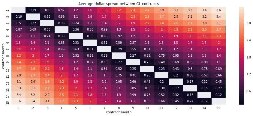
The further apart the contracts, the wider the spread. Adjacent contracts such as month 1 and 2 have average spreads of less than $0.30, while more distant contracts have spreads of up to $3.60. Larger average spreads might indicate larger divergences and re-convergences, possibly resulting in larger gross profits that could survive transaction costs.

Trade native spreads

The above backtest models trading non-native spreads. That is, buying or selling the calendar spread would involve a separate buy or sell order for each individual leg. This incurs a separate transaction cost for each leg. As an alternative, CL calendar spreads also trade natively on NYMEX. The native combo has its own bid and ask and can be bought or sold in a single transaction. While this still results in two commissions (one for each leg), the bid-ask spread is typically narrower than trading each leg separately.

The code repository link at the end of the article includes a demonstration of trading native calendar spreads.

Other ideas

Other ideas to reduce transaction costs include:

• Use limit orders to avoid paying the bid-ask spread. The above backtest uses market orders.
• Switch to a lower data frequency such as 1-hour bars. This will result in fewer trades and lower transaction costs.
• Use a longer rolling window for computing Bollinger Bands. This will make the bands wider and thus reduce the number of trades.
• Place the Bollinger Bands 3 standard deviations away instead of 2.

Conclusion

The challenges of intraday strategies differ from the challenges of end-of-day strategies. With end-of-day strategies, often the researcher's primary difficulty is to find a needle of meaningful alpha in the haystack of market randomness. With intraday strategies, it is often easier to find gross alpha, but the challenge is not to be swamped by the higher transaction costs associated with frequent trading. Intraday trading of crude oil calendar spreads offers a good illustration of this point.

Explore this research on your own

This research was created with QuantRocket. Clone the calspread repository to get the code and perform your own analysis.