Is There Alpha in Borrow Fees?
Wed May 15 2024 by Brian StanleyBorrow fees reflect how likely short sellers think a stock is to decline. Can this information be incorporated into trading strategies as an alpha factor? This article uses Alphalens to explore the relationship between borrow fees and forward returns and uses Moonshot and Zipline to demonstrate ways to incorporate borrow fees into long or short strategies.
Summary
- High borrow fees are an indication that many short sellers think a stock will decline.
- Short sellers are right: stocks with high borrow fees tend to decline.
- High borrow fees largely offset the profits from shorting high borrow fee stocks, limiting the alpha potential of short strategies.
- Long investors can improve returns by avoiding stocks with high borrow fees.
What are Borrow Fees?
Borrow fees, also known as stock loan fees, are the fees short sellers pay to stock owners to borrow shares they wish to sell short. The payment is typically split between the stock owner whose shares are loaned out and the broker who facilitates the loan.
The amount that short sellers pay is a variable percentage of the dollar value of the loaned shares. Borrow fees are quoted as annualized interest rates but are assessed daily. For example, a short seller who borrows $100,000 worth of shares at an annualized interest rate of 1% will be assessed a daily fee of 1/360th of 1 percent of $100,000, or $2.78 per day.
Fees can range widely, from as low as 0.25% (25 basis points) per year for easy-to-borrow stocks up to 100% or more for hard-to-borrow stocks. The fees are determined by supply and demand: the more traders want to short a stock, the higher the fee. Consequently, borrow fees are a useful indicator of the collective sentiment of short sellers about any particular stock.
QuantRocket maintains an archive of historical borrow fees for US and global stocks dating back to 2018. The data are sourced from Interactive Brokers and are updated daily.
Alphalens Analysis
Short sellers are typically considered to be informed market participants, aka smart money. If high borrow fees mean that short sellers think that a stock is overvalued or a company is in trouble, can we use that information as a source of alpha?
To find out, I first turn to Pipeline and Alphalens to analyze the relationship between borrow fees and forward returns for US stocks. I begin by creating a Pipeline with two columns: daily borrow fees for all common stocks, and dollar volume quantiles (as a proxy for size). I exclude microcaps, defined here as the bottom 25% by dollar volume, due to their atypical characteristics that can obscure underlying trends.
from zipline.pipeline import Pipeline, ibkr, master
from zipline.pipeline.factors import AverageDollarVolume

# limit analysis to common stocks
universe = master.SecuritiesMaster.usstock_SecurityType2.latest.eq("Common Stock")

borrow_fee = ibkr.BorrowFees.FeeRate.latest

avg_dollar_volume = AverageDollarVolume(window_length=90)

pipeline = Pipeline(
    columns={
        "borrow_fee": borrow_fee,
        "size": avg_dollar_volume.quantiles(4)
    },
    initial_universe=universe,
    screen=(
        # ignore microcaps
        avg_dollar_volume.percentile_between(26, 100)
    )
)
I pass the Pipeline to Alphalens, partitioning stocks at the 50th, 75th, and 90th percentiles by borrow fee:
import alphalens as al

al.from_pipeline(
    pipeline,
    start_date="2018-04-16", # this is the start date of the borrow fees data
    end_date="2024-04-30",
    factor="borrow_fee",
    groupby="size",
    quantiles=[0, 0.5, 0.75, 0.9, 1], # split at 50th, 75th, and 90th percentile
    relative_returns=False, # Alphalens shows relative and absolute returns by default, let's ignore relative
    segment="Y"
)
Results
Stocks with high borrow fees perform worse than stocks with low borrow fees. In the bar plot, we see that while most US stocks had positive returns since 2018, the decile of stocks with the highest borrow fees (quantile 4) had negative returns. The line plot below the bar plot shows the cumulative performance of a factor-weighted portfolio that weights positions proportionally to their borrow fees. A portfolio concentrated in high borrow fee stocks would have steadily declined since 2018. It appears that short sellers are skillful at identifying stocks that are likely to underperform.
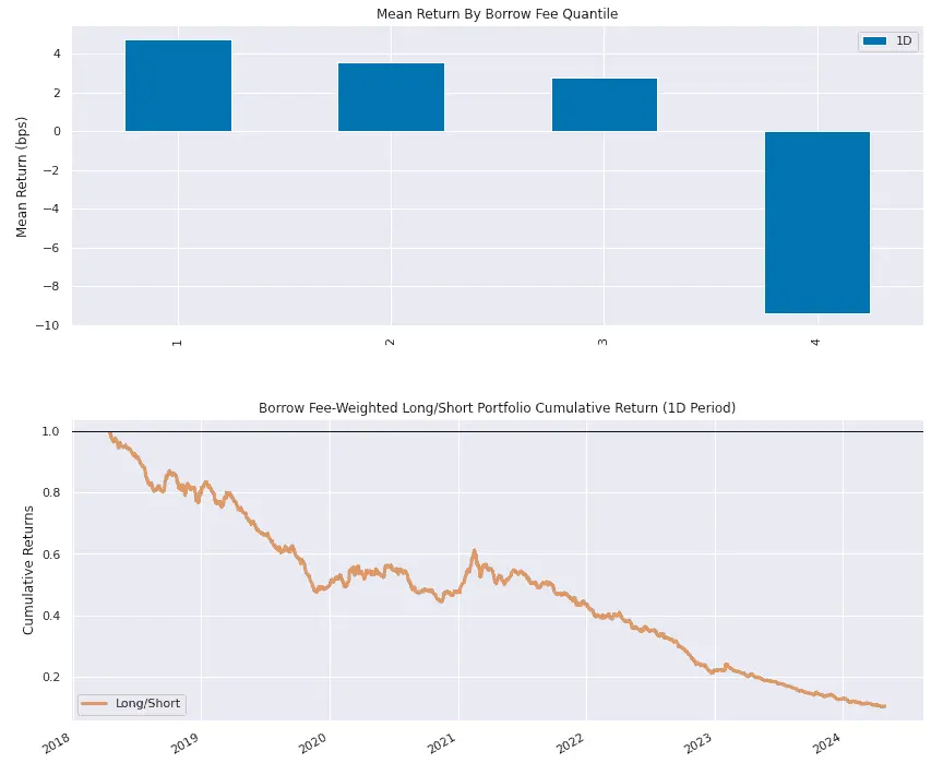
Line plot (bottom): Cumulative performance of borrow fee-weighted portfolio (higher borrow fees = larger positions).
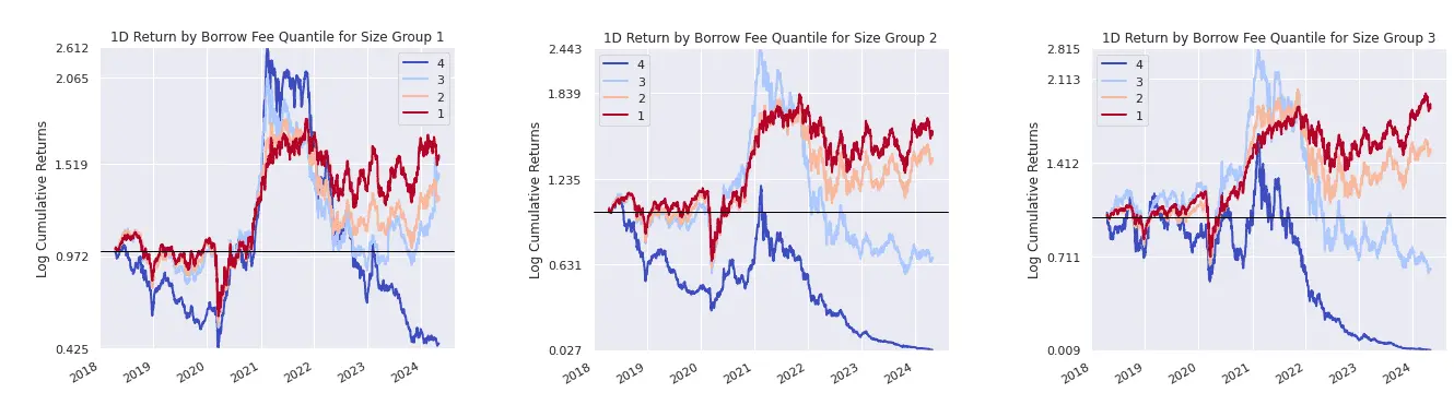
The following subplots analyze the relationship between borrow fees and forward returns by company size (using dollar volume as a proxy for company size). The leftmost plot analyzes smallcaps (group 1), the middle plot analyzes midcaps (group 2), and the rightmost plot analyzes largecaps (group 3). In each plot, stocks with the highest borrow fees (borrow fee quantile 4, blue line) perform worst.
Should We Short Stocks with High Borrow Fees?
Given that stocks with high borrow fees tend to decline, can we make money by shorting a portfolio of high borrow fee stocks? We will benefit from the stocks' declines but will have to pay high fees to borrow them. Which effect will dominate?
To find out, I use Moonshot to backtest a strategy that shorts stocks in the highest borrow fee decile, and I use Moonshot's built-in IBKRBorrowFees class to debit borrowing costs. Highlights of the Moonshot strategy are shown below:
from quantrocket.fundamental import get_ibkr_borrow_fees_reindexed_like
from quantrocket.master import get_securities_reindexed_like
class HighBorrowShort(Moonshot):
...
SLIPPAGE_CLASSES = IBKRBorrowFees
def prices_to_signals(self, prices: pd.DataFrame):
...
# rank by borrow fee and short the 10% with the highest fees
borrow_fees = get_ibkr_borrow_fees_reindexed_like(closes)
borrow_fee_ranks = borrow_fees.rank(axis=1, ascending=False, pct=True)
short_signals = borrow_fee_ranks <= 0.10
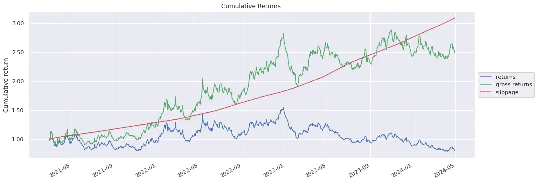
return -short_signals.astype(int)The cumulative return plot reveals that the strategy is profitable on a gross basis (green line), but the high borrow fees (red line) eat up the profits and result in a roughly flat net performance (blue line). It seems that while short sellers can accurately predict which stocks will decline, they have difficulty profiting from their knowledge due to competition from other short sellers who drive up borrow costs. This is a good example of the limits to arbitrage.
Using Borrow Fees as a Filter in Long Strategies
Although borrowing costs make it difficult for short sellers to turn their insights into profits, long investors have it easier. Since they don't incur borrowing costs, they can benefit from the insights of short sellers by avoiding owning stocks with high borrow fees. In this way, short sellers function as research analysts for long portfolio managers, advising them of stocks to exclude from their portfolios.
Using Zipline, I create a simple long-only strategy that buys an equal-weighted portfolio of midcap stocks (defined here as stocks in the 50th-75th percentile by dollar volume) excluding stocks with borrow fees above 0.3%:
MAX_BORROW_FEE = 0.3
def make_pipeline():
...
screen = AverageDollarVolume(window_length=90).percentile_between(50, 75)
if MAX_BORROW_FEE:
screen &= (ibkr.BorrowFees.FeeRate.latest <= MAX_BORROW_FEE)
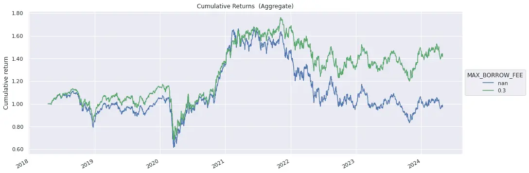
...I run a parameter scan to test the strategy with and without the borrow fee filter. The portfolio that excludes high borrow fee stocks (green line) outperforms the portfolio that does not exclude them (blue line).
Conclusion
Short sellers are skilled at identifying stocks that are likely to decline, as evidenced by the negative relationship between borrow fees and forward returns. However, when short sellers attempt to profit from their predictions by shorting these stocks, they drive up borrow fees, which eats up their profit. Long portfolio managers are best positioned to benefit from the insights of short sellers by avoiding stocks with high borrow fees.
Explore this research on your own
This research was created with QuantRocket. Clone the borrow-fees-alpha repository to get the code and perform your own analysis.
quantrocket codeload clone 'borrow-fees-alpha'About QuantRocket
QuantRocket is a Python-based platform for researching, backtesting, and trading quantitative strategies. It provides a JupyterLab environment, offers a suite of data integrations, and supports multiple backtesters: Zipline, the open-source backtester that originally powered Quantopian; Alphalens, an alpha factor analysis library; Moonshot, a vectorized backtester based on pandas; and MoonshotML, a walk-forward machine learning backtester. Built on Docker, QuantRocket can be deployed locally or to the cloud and has an open architecture that is flexible and extensible.
Learn more or install QuantRocket now to get started.
 Send a Message