For installation instructions, please see the Installation tutorial for your platform.
License key
Activation
To activate QuantRocket, look up your license key on your account page and enter it in your deployment:
$ quantrocket license set'XXXXXXXXXXXXXXXX'
>>> from quantrocket.license import set_license
>>> set_license("XXXXXXXXXXXXXXXX")
$ curl -X PUT 'http://houston/license-service/license/XXXXXXXXXXXXXXXX'
View your license
You can view the details of the currently installed license:
$ quantrocket license get
licensekey: XXXX....XXXX
software_license:
  account:
    account_limit: XXXXXX USD
  concurrent_install_limit: XX
  license_type: Professional
  user_limit: XX
The license service will re-query your subscriptions and permissions every 10 minutes. If you make a change to your billing plan and want your deployment to see the change immediately, you can force a refresh:
$ quantrocket license get --force-refresh
>>> from quantrocket.license import get_license_profile
>>> get_license_profile(force_refresh=True)
$ curl -X GET 'http://houston/license-service/license?force_refresh=true'
Account limit validation
The account limit displayed in your license profile output applies to live trading using the blotter and to real-time data. The account limit does not apply to historical data collection, research, or backtesting. For advisor accounts, the account size is the sum of all master and sub-accounts.
Paper trading is not subject to the account limit, however paper trading requires that the live account limit has previously been validated. Thus before paper trading it is first necessary to connect your live account at least once and let the software validate it.
To validate your account limit if you have only connected your paper account:
Wait approximately 1 minute. The software queries your account balance every minute whenever your broker is connected.
To verify that account validation has occurred, refresh your license profile. It should now display your account balance and whether the balance is under the account limit:
$ quantrocket license get --force-refresh
licensekey: XXXX....XXXX
software_license:
  account:
    account_balance: 593953.42 USD
    account_balance_details:
    - Account: U12345
      Currency: USD
      NetLiquidation: 593953.42 USD
    account_balance_under_limit: true
    account_limit: XXXXXX USD
  concurrent_install_limit: XX
  license_type: Professional
  user_limit: XX
If the command output is missing the account_balance and account_balance_under_limit keys, this indicates that the account limit has not yet been validated.
Now you can switch back to your paper account and begin paper trading.
User limit vs concurrent install limit
The output of your license profile displays your user limit and your concurrent install limit. User limit indicates the total number of distinct users who are licensed to use the software in any given month. Concurrent install limit indicates the total number of copies of the software that may be installed and running at any given time.
The concurrent install limit is set to (user limit + 1).
Rotate license key
You can rotate your license key at any time from your account page.
Connect from other applications
If you run other applications, you can connect them to your QuantRocket deployment for the purpose of querying data, submitting orders, etc.
Each remote connection to a cloud deployment counts against your plan's concurrent install limit. For example, if you run a single cloud deployment of QuantRocket and connect to it from a single remote application, this is counted as 2 concurrent installs, one for the deployment and one for the remote connection. (Connecting to a local deployment from a separate application running on your local machine does not count against the concurrent install limit.)
To utilize the Python API and/or CLI from outside of QuantRocket, install the client on the application or system you wish to connect from:
$ pip install 'quantrocket-client'
To ensure compatibility, the MAJOR.MINOR version of the client should match the MAJOR.MINOR version of your deployment. For example, if your deployment is version 2.1.x, you can install the latest 2.1.x client:
$ pip install 'quantrocket-client>=2.1,<2.2'
Don't forget to update your client version when you update your deployment version.
Next, set environment variables to tell the client how to connect to your QuantRocket deployment. For a cloud deployment, this means providing the deployment URL and credentials:
$# Linux/MacOS syntax:$export HOUSTON_URL=https://quantrocket.123capital.com$export HOUSTON_USERNAME=myusername$export HOUSTON_PASSWORD=mypassword
$# Windows syntax (restart PowerShell afterwards for change to take effect):$ [Environment]::SetEnvironmentVariable("HOUSTON_URL", "https://quantrocket.123capital.com", "User")$ [Environment]::SetEnvironmentVariable("HOUSTON_USERNAME", "myusername", "User")$ [Environment]::SetEnvironmentVariable("HOUSTON_PASSWORD", "mypassword", "User")
For connecting to a local deployment, only the URL is needed:
$# Linux/MacOS syntax:$export HOUSTON_URL=http://localhost:1969
$# Windows syntax (restart PowerShell afterwards for change to take effect):$ [Environment]::SetEnvironmentVariable("HOUSTON_URL", "http://localhost:1969", "User")
Environment variable syntax varies by operating system. Don't forget to make your environment variables persistent by adding them to .bashrc (Linux) or .profile (MacOS) and sourcing it (for example source ~/.bashrc), or restarting PowerShell (Windows).
Finally, test that it worked:
$ quantrocket houston ping
msg: hello from houston
>>> from quantrocket.houston import ping
>>> ping()
{u'msg': u'hello from houston'}
$ curl -u myusername:mypassword https://quantrocket.123capital.com/ping
{"msg": "hello from houston"}
To connect from applications running languages other than Python, you can skip the client installation and use the HTTP API directly.
Broker and Data Connections
This section outlines how to connect to brokers and third-party data providers.
Because QuantRocket runs on your hardware, third-party credentials and API keys that you enter into the software are secure. They are encrypted at rest and never leave your deployment. They are used solely for connecting directly to the third-party API.
Interactive Brokers
Connecting to Interactive Brokers requires an IBKR Pro account. IBKR Lite accounts do not provide API access and will not work with QuantRocket. To switch from IBKR Lite to IBKR Pro, log in to the Client Portal for your Interactive Brokers account.
IBKR Account Structure
Multiple logins and data concurrency
The structure of your Interactive Brokers (IBKR) account has a bearing on the speed with which you can collect real-time and historical data with QuantRocket. In short, the more IB Gateways you run, the more data you can collect. The basics of account structure and data concurrency are outlined below:
All interaction with the IBKR servers, including real-time and historical data collection, is routed through IB Gateway, IBKR's slimmed-down version of Trader Workstation.
IBKR imposes rate limits on the amount of historical and real-time data that can be received through IB Gateway.
Each IB Gateway is tied to a particular set of login credentials. Each login can be running only one active IB Gateway session at any given time.
However, an account holder can have multiple logins—at least two logins or possibly more, depending on the account structure. Each login can run its own IB Gateway session. In this way, an account holder can potentially run multiple instances of IB Gateway simultaneously.
QuantRocket is designed to take advantage of multiple IB Gateways. When running multiple gateways, QuantRocket will spread your market data requests among the connected gateways.
Since each instance of IB Gateway is rate limited separately by IBKR, the combined data throughput from splitting requests among two IB Gateways is twice that of sending all requests to one IB Gateway.
Each separate login must separately subscribe to the relevant market data in IBKR Client Portal.
Below are a few common ways to obtain additional logins.
IBKR account structures are complex and vary by subsidiary, local regulations, the person opening the account, etc. The following guidelines are suggestions only and may not be applicable to your situation.
Second user login
Individual account holders can add a second login to their account. This is designed to allow you to use one login for API trading while using the other login to use Trader Workstation for manual trading or account monitoring. However, you can use both logins to collect data with QuantRocket. Note that you can't use the same login to simultaneously run Trader Workstation and collect data with QuantRocket. However, QuantRocket makes it easy to start and stop IB Gateway on a schedule, so the following is an option:
Login 1 (used for QuantRocket only)
IB Gateway always running and available for data collection and placing API orders
Login 2 (used for QuantRocket and Trader Workstation)
automatically stop IB Gateway daily at 9:30 AM
Run Trader Workstation during trading session for manual trading/account monitoring
automatically start IB Gateway daily at 4:00 PM so it can be used for overnight data collection
Advisor/Friends and Family accounts
An advisor account or the similarly structured Friends and Family account offers the possibility to obtain additional logins. Even an individual trader can open a Friends and Family account, in which they serve as their own advisor. The account setup is as follows:
Master/advisor account: no trading occurs in this account. The account is funded only with enough money to cover market data costs. This yields 1 IB Gateway login.
Master/advisor second user login: like an individual account, the master account can create a second login, subscribe to market data with this login, and use it for data collection.
Client account: this is main trading account where the trading funds are deposited. This account receives its own login (for 3 total). By default this account does not having trading permissions, but you can enable client trading permissions via the master account, then subscribe to market data in the client account and begin using the client login to run another instance of IB Gateway. (Note that it's not possible to add a second login for a client account.)
If you have other accounts such as retirement accounts, you can add them as additional client accounts and obtain additional logins.
Paper trading accounts
Each IBKR account holder can enable a paper trading account for simulated trading. You can share market data with your paper account and use the paper account login with QuantRocket to collect data, as well as to paper trade your strategies. You don't need to switch to using your live account until you're ready for live trading (although it's also fine to use your live account login from the start).
Note that, due to restrictions on market data sharing, it's not possible to run IB Gateway using the live account login and corresponding paper account login at the same time. If you try, one of the sessions will disconnect the other session.
IBKR market data permissions
To collect IBKR data using QuantRocket, you must subscribe to the relevant market data in your IBKR account. In IBKR Client Portal, click on Settings > User Settings > Market Data Subscriptions:
Click the edit icon then select and confirm the relevant subscriptions:
Market data for paper accounts
IBKR paper accounts do not directly subscribe to market data. Rather, to access market data using your IBKR paper account, subscribe to the data in your live account and share it with your paper account. Log in to IBKR Client Portal with your live account login and go to Settings > Account Settings > Paper Trading Account:
Then select the option to share your live account's market data with your paper account:
IB Gateway
QuantRocket uses the IBKR API to collect market data from IBKR, submit orders, and track positions and account balances. All communication with IBKR is routed through IB Gateway, a Java application which is a slimmed-down version of Trader Workstation (TWS) intended for API use. You can run one or more IB Gateway services through QuantRocket, where each gateway instance is associated with a different IBKR username and password.
Connect to IBKR
Your credentials are encrypted at rest and never leave your deployment.
IB Gateway runs inside the ibg1 container and connects to IBKR using your IBKR username and password. (If you have multiple IBKR usernames, you can run multiple IB Gateways.) The ibgrouter container provides an API that allows you to start and stop IB Gateway inside the ibg container(s).
Secure Login System (Two-Factor Authentication)
Interactive Brokers requires two-factor authentication for most live accounts. Interactive Brokers supports several different methods of two-factor authentication, but to use IB Gateway with QuantRocket you should enroll in mobile authentication, which involves receiving a notification on your mobile device to complete login.
Be sure to read the section about IB Gateway auto-restarts which outlines the need to perform two-factor authentication weekly on Sundays. You will also need to perform two-factor authentication any time you log back in to IB Gateway after having logged out, regardless of the day. You can set up alerts to avoid missing two-factor notifications on your mobile device.
Two-factor authentication is not required for paper accounts. For the convenience of omitting two-factor authentication, and as a general best practice, you can log into a paper account for data collection and only log into a live account when you are ready for live trading.
Enter IBKR login
To connect to your IBKR account, enter your IBKR login into your deployment, as well as the desired trading mode (live or paper). You'll be prompted for your password:
$ quantrocket ibg credentials 'ibg1' --username 'myuser' --paper # or --live
Enter IBKR Password:
status: successfully set ibg1 credentials
>>> from quantrocket.ibg import set_credentials
>>> set_credentials("ibg1", username="myuser", trading_mode="paper")
Enter IBKR Password:
{'status': 'successfully set ibg1 credentials'}
$ curl -X PUT 'http://houston/ibg1/credentials' -d 'username=myuser' -d 'password=mypassword' -d 'trading_mode=paper'
{"status": "successfully set ibg1 credentials"}
When setting your credentials, QuantRocket securely stores your credentials inside your deployment so you don't need to enter them again, then starts IB Gateway to verify that your credentials work. Starting IB Gateway takes approximately 30 seconds.
If you are connecting to a live IBKR account that requires second factor authentication, you will see an error message:
$ quantrocket ibg credentials 'ibg1' --username 'myuser' --live
Enter IBKR Password:
msg: Second factor authentication required to complete login, please check your mobile
  device for a notification. See http://qrok.it/h/ib2fa for help.
status: error
>>> from quantrocket.ibg import set_credentials
>>> set_credentials("ibg1", username="myuser", trading_mode="live")
Enter IBKR Password:
HTTPError: ('401 Client Error: UNAUTHORIZED for url: http://houston/ibg1/credentials', {'status': 'error', 'msg': 'Second factor authentication required to complete login, please check your mobile device for a notification. See http://qrok.it/h/ib2fa for help.'})
$ curl -X PUT 'http://houston/ibg1/credentials' -d 'username=myuser' -d 'password=mypassword' -d 'trading_mode=live'
{"status": "error", "msg": "Second factor authentication required to complete login, please check your mobile device for a notification. See http://qrok.it/h/ib2fa for help."}
Complete the authentication using your mobile device. If you fail to complete authentication within 3 minutes, QuantRocket will stop and restart IB Gateway, resulting in a new mobile notification. This process will repeat indefinitely until you complete the authentication.
If you encounter errors trying to start IB Gateway, refer to a later section to learn how to access the IB Gateway GUI for troubleshooting.
Querying your IBKR account balance is a good way to verify your IBKR connection:
When you sign up for an IBKR paper account, IBKR provides login credentials for the paper account. However, it is also possible to login to the paper account by using your live account credentials and specifying the trading mode as "paper". Thus, technically the paper login credentials are unnecessary.
Using your live login credentials for both live and paper trading allows you to easily switch back and forth. Supposing you originally select the paper trading mode:
$ quantrocket ibg credentials 'ibg1' --username 'myliveuser' --paper
Enter IBKR Password:
status: successfully set ibg1 credentials
>>> from quantrocket.ibg import set_credentials
>>> set_credentials("ibg1", username="myliveuser", trading_mode="paper")
Enter IBKR Password:
{'status': 'successfully set ibg1 credentials'}
$ curl -X PUT 'http://houston/ibg1/credentials' -d 'username=myliveuser' -d 'password=mypassword' -d 'trading_mode=paper'
{"status": "successfully set ibg1 credentials"}
You can later switch to live trading mode without re-entering your credentials:
$ quantrocket ibg credentials 'ibg1' --live
msg: Second factor authentication required to complete login, please check your mobile
  device for a notification. See http://qrok.it/h/ib2fa for help.
status: error
>>> set_credentials("ibg1", trading_mode="live")
HTTPError: ('401 Client Error: UNAUTHORIZED for url: http://houston/ibg1/credentials', {'status': 'error', 'msg': 'Second factor authentication required to complete login, please check your mobile device for a notification. See http://qrok.it/h/ib2fa for help.'})
$ curl -X PUT 'http://houston/ibg1/credentials' -d 'trading_mode=live'
{"status": "error", "msg": "Second factor authentication required to complete login, please check your mobile device for a notification. See http://qrok.it/h/ib2fa for help."}
If you forget which mode you're in (or which login you used), you can check:
$ quantrocket ibg credentials 'ibg1'
TRADING_MODE: live
TWSUSERID: myliveuser
$ curl -X GET 'http://houston/ibg1/credentials'
{"TWSUSERID": "myliveuser", "TRADING_MODE": "live"}
Start/stop IB Gateway
IB Gateway must be running whenever you want to collect market data or place or monitor orders. You can optionally stop IB Gateway when you're not using it. Interactive Brokers limits each unique IBKR login to one IB Gateway or Trader Workstation session at a time. Therefore, if you need to log in to Trader Workstation using the same login credentials you are using with QuantRocket, you must first stop IB Gateway.
To check the current status of your IB Gateway(s):
$ quantrocket ibg status
ibg1: stopped
>>> from quantrocket.ibg import list_gateway_statuses
>>> list_gateway_statuses()
{'ibg1': 'stopped'}
$ curl -X GET 'http://houston/ibgrouter/gateways'
{"ibg1": "stopped"}
You can start IB Gateway, optionally waiting for the startup process (and mobile authentication, if applicable) to complete:
IB Gateway automatically restarts itself once a day. This behavior is enforced by IB Gateway itself, not QuantRocket, and is designed to keep IB Gateway running smoothly.
The daily restart happens at 11:45 PM New York time. The restart takes about 30 seconds. If historical or fundamental data collection is in progress, the data collection services will detect the interrupted connection and automatically resume when the connection is restored. (If IB Gateway is not running at the time of the restart, no restart is required or occurs.)
If you need the restart to occur at a different time (for example because your strategy may be placing trades at 11:45 PM New York time), you can modify the restart time by opening the IB Gateway GUI and navigating to Configure > Settings > Lock and Exit. Each time you re-deploy QuantRocket or run a software update which creates or re-creates the ibg1 container, you will need to edit the setting again.
Alternatively, to avoid the need to edit the setting each time you re-deploy the ibg1 container, you can add an AUTO_RESTART_TIME environment variable to your docker-compose.override.yml, which should specify the New York time in HH:MM format when you want the daily restart to occur:
# docker-compose.override.ymlservices: ibg1: environment: AUTO_RESTART_TIME:'21:00'# 9:00 PM New York time
Then, re-deploy the ibg1 service:
$cd /path/to/docker-compose.yml$ docker compose -p quantrocket up -d ibg1
You can learn more about docker-compose.override.yml in another section.
Auto-restart with two-factor authentication
For live accounts with two-factor authentication, the Sunday auto-restart will require two-factor authentication. On other days, the auto-restart will automatically log you back in without the need to perform two-factor authentication. Thus, accounts with two-factor authentication can remain logged in all week, with mobile authentication on Sundays.
The restart will happen automatically and you will only need to acknowledge the mobile notification to complete the login; thus you won't need access to QuantRocket itself. If you miss the mobile notification, QuantRocket will stop and restart IB Gateway every 3 minutes to trigger a new notification, until you eventually acknowledge one.
The timing of the daily auto-restart determines what time you will receive two-factor authentication notifications on your mobile device on Sunday. The default time is 11:45 PM New York time. You can adjust this time by setting the AUTO_RESTART_TIME environment variable as shown above. Ideally, you should choose an auto-restart time that will be convenient for acknowledging two-factor authentication notifications on Sunday, and that won't interrupt any live trading on other days of the week.
Two-Factor Authentication alerts
Two-factor authentication notifications from the IBKR mobile app are typically silent: a banner will appear on your mobile device but no sound will play. This can result in missed notifications if you are not expecting a notification, as may be the case when the weekly auto-restart occurs.
You can use QuantRocket's Papertrail integration to generate a sound when two-factor authentication is required, to decrease the chance of missing a notification. Each time a two-factor notification is sent to your mobile device, a message will be logged to flightlog:
quantrocket.ibg1 WARNING Second factor authentication required to complete login, please check your mobile device for a notification. See http://qrok.it/h/ib2fa for help.
Setting up the Papertrail integration will cause this message to appear in Papertrail as well. Then, you can create an alert in Papertrail that monitors for the phrase "Second factor authentication required" and, when found, sends a notification to one of Papertrail's integrated notification services such as Pushover. Pushover will send its own notification to your device that will play a sound, drawing your attention to the two-factor notification from IBKR.
IB Gateway GUI
Normally you won't need to access the IB Gateway GUI. However, you might need access to troubleshoot a login issue.
To allow access to the IB Gateway GUI, QuantRocket uses NoVNC, which uses the WebSockets protocol to support VNC connections in the browser. To open an IB Gateway GUI connection in your browser, click the "IB Gateway GUI" button located on the JupyterLab Launcher or from the File menu. The IB Gateway GUI will open in a new window (make sure your browser doesn't block the pop-up).
If IB Gateway isn't currently running, the screen will be black.
To quit the VNC session but leave IB Gateway running, simply close your browser tab.
For improved security for cloud deployments, QuantRocket doesn't directly expose any VNC ports to the outside. By proxying VNC connections through houston using NoVNC, such connections are protected by Basic Auth and SSL, just like every other request sent through houston.
Multiple IB Gateways
QuantRocket support running multiple IB Gateways, each associated with a particular IBKR login. Two of the main reasons for running multiple IB Gateways are:
The default IB Gateway service is called ibg1. To run multiple IB Gateways, create a file called docker-compose.override.yml in the same directory as your docker-compose.yml and add the desired number of additional services as shown below. In this example we are adding two additional IB Gateway services, ibg2 and ibg3, which inherit from the definition of ibg1:
You can learn more about docker-compose.override.yml in another section.
Then, deploy the new service(s):
$cd /path/to/docker-compose.yml$ docker compose -p quantrocket up -d
You can then enter your login for each of the new IB Gateways:
$ quantrocket ibg credentials 'ibg2' --username 'myuser' --paper
Enter IBKR Password:
status: successfully set ibg2 credentials
>>> from quantrocket.ibg import set_credentials
>>> set_credentials("ibg2", username="myuser", trading_mode="paper")
Enter IBKR Password:
{'status': 'successfully set ibg2 credentials'}
$ curl -X PUT 'http://houston/ibg2/credentials' -d 'username=myuser' -d 'password=mypassword' -d 'trading_mode=paper'
{"status": "successfully set ibg2 credentials"}
When starting and stopping gateways, the default behavior is start or stop all gateways. To target specific gateways, use the gateways parameter:
$ quantrocket ibg start --gateways 'ibg2'
status: the gateways will be started asynchronously
>>> from quantrocket.ibg import start_gateways
>>> start_gateways(gateways=["ibg2"])
{'status': 'the gateways will be started asynchronously'}
$ curl -X POST 'http://houston/ibgrouter/gateways?gateways=ibg2'
{"status": "the gateways will be started asynchronously"}
Market data permission file
Generally, loading your market data permissions into QuantRocket is only necessary when you are running multiple IB Gateway services with different market data permissions for each.
To retrieve market data from IBKR, you must subscribe to the appropriate market data subscriptions in IBKR Client Portal. QuantRocket can't identify your subscriptions via API, so you must tell QuantRocket about your subscriptions by loading a YAML configuration file. If you don't load a configuration file, QuantRocket will assume you have market data permissions for any data you request through QuantRocket. If you only run one IB Gateway service, this is probably sufficient and you can skip the configuration file. However, if you run multiple IB Gateway services with separate market data permissions for each, you will probably want to load a configuration file so QuantRocket can route your requests to the appropriate IB Gateway service. You should also update your configuration file whenever you modify your market data permissions in IBKR Client Portal.
An example IB Gateway permissions template is available from the JupyterLab launcher.
QuantRocket looks for a market data permission file called quantrocket.ibg.permissions.yml in the top-level of the Jupyter file browser (that is, /codeload/quantrocket.ibg.permissions.yml). The format of the YAML file is shown below:
# each top-level key is the name of an IB Gateway serviceibg1:# list the exchanges, by security type, this gateway has permission for marketdata: STK: -NYSE -ISLAND -TSEJ FUT: -CME -OSE CASH: -IDEALPRO# Include a separate section for each IB Gateway serviceibg2: marketdata: STK: -NYSE
When you create or edit this file, QuantRocket will detect the change and load the configuration. It's a good idea to have flightlog open when you do this. If the configuration file is valid, you'll see a success message:
quantrocket.ibgrouter: INFO Successfully loaded /codeload/quantrocket.ibg.permissions.yml
If the configuration file is invalid, you'll see an error message:
quantrocket.ibgrouter: ERROR Could not load /codeload/quantrocket.ibg.permissions.yml:
quantrocket.ibgrouter: ERROR unknown key(s) for service ibg1: marketdata-typo
You can also dump out the currently loaded config to confirm it is as you expect:
There are two types of logs produced by IB Gateway: API logs and Gateway logs. The API logs show the API messages being sent back and forth between QuantRocket and IB Gateway. The Gateway logs show detailed debugging logs for the IB Gateway application.
The API logs are occasionally useful for troubleshooting QuantRocket and might be requested by QuantRocket support. The Gateway logs might occasionally be requested by Interactive Brokers support. If you need to send these files to QuantRocket or Interactive Brokers support for troubleshooting, you can generate and export the files as described below.
API logs
You can use the IB Gateway GUI to generate API logs, then export the logs to the Docker filesystem, then copy them to your local filesystem.
In the IB Gateway GUI, click Configure > Settings, navigate to API > Settings and check the box for "Create API message log file."
IB Gateway will begin to generate API logs. Continue using the application until the messages you are interested in have been generated.
Next, in the IB Gateway GUI, click File > API Logs, and select the day you're interested in.
Click Export Logs or Export Today Logs. A file browser will open, showing the filesystem inside the Docker container.
Export the log file to an easy-to-find location such as /tmp/api-exported-logs.txt.
From the host machine, copy the exported logs from the Docker container to your local filesystem. For ibg1 logs saved to the above location, the command would be:
In the IB Gateway GUI, click File > Gateway Logs, and select the day you're interested in.
Click Export Logs or Export Today Logs. A file browser will open, showing the filesystem inside the Docker container.
Export the log file to an easy-to-find location such as /tmp/ibgateway-exported-logs.txt.
From the host machine, copy the exported logs from the Docker container to your local filesystem. For ibg1 logs saved to the above location, the command would be:
Your credentials are encrypted at rest and never leave your deployment.
You can connect to one or more paper Alpaca accounts and one or more live Alpaca accounts. Enter your API key and trading mode for each account you want to connect (you will be prompted for your secret key):
$ quantrocket license alpaca-key --api-key 'PXXXXXXXXXXXXXXXXXX' --paper
Enter Alpaca secret key:
status: successfully set Alpaca paper API key
>>> from quantrocket.license import set_alpaca_key
>>> set_alpaca_key(api_key="PXXXXXXXXXXXXXXXXXX", trading_mode="paper")
Enter Alpaca secret key:
{'status': 'successfully set Alpaca paper API key'}
$ curl -X PUT 'http://houston/license-service/credentials/alpaca' -d 'api_key=PXXXXXXXXXXXXXXXXXX&secret_key=XXXXXXXXXXXXXXXXXX&trading_mode=paper'
{"status": "successfully set Alpaca paper API key"}
If you plan to use Alpaca for real-time data and subscribe to Alpaca's unlimited data package which provides access to the full SIP data feed, you can indicate this by including the --realtime-data/realtime_data parameter and specifying 'sip' (if omitted, only Alpaca's free IEX data permission is assumed):
$ quantrocket license alpaca-key --api-key 'XXXXXXXXXXXXXXXXXX' --live --realtime-data 'sip'
Enter Alpaca secret key:
status: successfully set Alpaca live API key
>>> set_alpaca_key(api_key="XXXXXXXXXXXXXXXXXX", trading_mode="live", realtime_data="sip")
Enter Alpaca secret key:
{'status': 'successfully set Alpaca live API key'}
$ curl -X PUT 'http://houston/license-service/credentials/alpaca' -d 'api_key=XXXXXXXXXXXXXXXXXX&secret_key=XXXXXXXXXXXXXXXXXX&trading_mode=live&realtime_data=sip'
{"status": "successfully set Alpaca live API key"}
You can view the currently configured API keys, which are organized by account number:
$ quantrocket license alpaca-key
12345678:
api_key: XXXXXXXXXXXXXXXXXX
realtime_data: sip
trading_mode: live
P1234567:
api_key: PXXXXXXXXXXXXXXXXXX
realtime_data: iex
trading_mode: paper
To later change your real-time data permission, simply re-enter the credentials with the new permission:
$ quantrocket license alpaca-key --api-key 'XXXXXXXXXXXXXXXXXX' --live --realtime-data 'iex'
Enter Alpaca secret key:
status: successfully set Alpaca live API key
>>> set_alpaca_key(api_key="XXXXXXXXXXXXXXXXXX", trading_mode="live", realtime_data="iex")
Enter Alpaca secret key:
{'status': 'successfully set Alpaca live API key'}
$ curl -X PUT 'http://houston/license-service/credentials/alpaca' -d 'api_key=XXXXXXXXXXXXXXXXXX&secret_key=XXXXXXXXXXXXXXXXXX&trading_mode=live&realtime_data=iex'
{"status": "successfully set Alpaca live API key"}
Alpaca account reset
Since you can connect to multiple Alpaca accounts, adding new credentials does not remove old credentials. If you reset your Alpaca paper account or otherwise change account numbers and your previously entered credentials are no longer valid, you may see errors in the logs for your old account:
quantrocket.blotter: WARNING Error connecting to Alpaca, will try again shortly: 403 Client Error: Forbidden for url: https://paper-api.alpaca.markets/v2/orders?limit=500&direction=asc&status=open
Although there is no API command for removing old credentials, you can delete the encrypted credentials file from the license-service container like this:
>>> from quantrocket.license import get_polygon_key
>>> get_polygon_key()
{'api_key': 'XXXXXXXXXXXXXXXXXX'}
curl -X GET 'http://houston/license-service/credentials/polygon'
{"api_key": "XXXXXXXXXXXXXXXXXX"}
Nasdaq Data Link (Quandl)
Nasdaq acquired Quandl in 2018 and rebranded Quandl as Nasdaq Data Link in 2021. However, QuantRocket APIs reflect the original Quandl branding.
Your credentials are encrypted at rest and never leave your deployment.
Users who subscribe to Sharadar data through Nasdaq Data Link (formerly Quandl) can access Sharadar data in QuantRocket. To enable access, enter your Nasdaq/Quandl API key:
$ quantrocket license quandl-key 'XXXXXXXXXXXXXXXXXX'
status: successfully set Quandl API key
>>> from quantrocket.license import set_quandl_key
>>> set_quandl_key(api_key="XXXXXXXXXXXXXXXXXX")
{'status': 'successfully set Quandl API key'}
$ curl -X PUT 'http://houston/license-service/credentials/quandl' -d 'api_key=XXXXXXXXXXXXXXXXXX'
{"status": "successfully set Quandl API key"}
>>> from quantrocket.license import get_quandl_key
>>> get_quandl_key()
{'api_key': 'XXXXXXXXXXXXXXXXXX'}
curl -X GET 'http://houston/license-service/credentials/quandl'
{"api_key": "XXXXXXXXXXXXXXXXXX"}
IDEs and Editors
JupyterLab is the primary user interface for QuantRocket and provides an ideal environment for interactive research. Alternatively, users who feel more at home in Visual Studio Code can connect it to QuantRocket with some basic setup.
JupyterLab
See the QuickStart for a hands-on overview of JupyterLab.
Data Browser
The Data Browser is a graphical tool for browsing the securities master database, price and fundamental data, and Pipeline output. With the Data Browser, you can:
Look up a financial instrument's exchange, contract specifications, or Sid (security ID) without querying the API.
View price charts for any of the securities in any of your historical price databases (including custom databases).
View time series plots of fundamental metrics (EPS, P/B ratio, etc) from Sharadar for US stocks.
Open DataFrames of securities or CSV files of securities returned by other QuantRocket APIs and explore the securities graphically. For example, open a CSV file of orders from a Moonshot or Zipline trading strategy to see what stocks will be traded.
Open Pipeline output to view the securities that passed your Pipeline screen and to view time series plots of Pipeline columns.
The Data Browser is accessible from the JupyterLab Launcher. For the integration with Pipeline, see the Pipeline tutorial in the Code Library.
If desired, you can install Visual Studio Code on your desktop and attach it to your local or cloud deployment. This allows you to edit code and open terminals from within VS Code. VS Code utilizes the environment provided by the QuantRocket container you attach to, so autocomplete and other features are based on the QuantRocket environment, meaning there's no need to manually replicate QuantRocket's environment on your local computer.
Follow these steps to use VS Code with QuantRocket.
In VS Code, open the extension manager and install the following extensions:
Python
Pylance
Docker
Dev Containers
Jupyter
For cloud deployments only: By default, VS Code will be able to see any Docker containers running on your local machine. To make VS Code see your QuantRocket containers running remotely in the cloud, run docker context use cloud, just as you would to deploy QuantRocket to the cloud. This command points Docker to the remote host where you are running QuantRocket and causes VS Code to see the containers running remotely. (Alternatively, you can change the Docker context from the Contexts section of the Docker panel in VS Code.)
Open the Docker panel in the side bar, find the jupyter container, right-click, and choose "Attach Visual Studio Code". A new window opens.
(The original VS Code window still points to your local computer and can be used to edit your local projects.)
The new VS Code window that opened is attached to the jupyter container. VS code will automatically install itself on the jupyter container.
Any extensions you may have installed on your local VS Code are not automatically installed on the remote VS Code, so you should install them. Open the Extensions Manager and install, at minimum, the Python extension, and anything else you like. VS Code remembers what you install in a local configuration file and restores your desired environment in the future even if you destroy and re-create the container.
In the Explorer window, click Open Folder, type 'codeload', then Open Folder. The files on your jupyter container will now be displayed in the VS Code file browser.
Jupyter notebooks in VS Code
If you open a Jupyter notebook in VS Code and execute a cell, you will be prompted to enter the URL of a Jupyter server. Enter http://houston/jupyter. When prompted for the Python interpreter to use, choose /opt/conda/bin/python.
Support for running Jupyter notebooks in VS Code is experimental. If you encounter problems starting notebooks in VS Code, please use JupyterLab instead.
Terminal utilities
.zshrc
You can add JupyterLab Terminal shortcuts by creating a .zshrc file and storing it at /codeload/.zshrc. This file will be run when you open a new terminal, just like on a standard Linux distribution. (zshrc stands for ZShell Run Commands file, where Z Shell is the shell used by QuantRocket's JupyterLab Terminal.)
A sample .zshrc file can be created from the JupyterLab Launcher.
A common use is to create aliases for commonly typed commands. For example, placing the following alias in your /codeload/.zshrc file will allow you to check your balance by simply typing balance:
alias balance="quantrocket account balance -l -f NetLiquidation | csvlook"
You can create aliases to custom scripts to get easy access to any commonly used functionality you want:
# run myfunction in /codeload/scripts/myscript.pyalias myscript="quantrocket satellite exec codeload.scripts.myscript.myfunction"
An alias can't accept arguments, so if you need to pass arguments to your script, you can instead define a shell function that executes the script and passes arguments:
# run myfunction in /codeload/scripts/myscript.py and pass an argumentfunction myscript {
quantrocket satellite exec codeload.scripts.myscript.myfunction --params myparam:$1
}
Here, the variable $1 will contain the first argument passed to your script. This script could be called with the parameter "someparam" as follows:
myscript someparam
After adding or editing a .zshrc file, you must open a new Terminal for the changes to take effect.
csvkit
Many QuantRocket API endpoints return CSV files. csvkit is a suite of utilities that makes it easier to work with CSV files from the command line. To make a CSV file more easily readable, use csvlook:
$ quantrocket master get --exchanges 'XNAS''XNYS' | csvlook -I
| Sid | Symbol | Exchange | Country | Currency | SecType | Etf | Timezone | Name |
| -------------- | ------ | -------- | ------- | -------- | ------- | --- | ------------------- | -------------------------- |
| FIBBG000B9XRY4 | AAPL | XNAS | US | USD | STK | 0 | America/New_York | APPLE INC |
| FIBBG000BFWKC0 | MON | XNYS | US | USD | STK | 0 | America/New_York | MONSANTO CO |
| FIBBG000BKZB36 | HD | XNYS | US | USD | STK | 0 | America/New_York | HOME DEPOT INC |
| FIBBG000BMHYD1 | JNJ | XNYS | US | USD | STK | 0 | America/New_York | JOHNSON & JOHNSON |
Another useful utility is csvgrep, which can be used to filter CSV files on fields not natively filterable by QuantRocket's API:
$# save a CSV of NYSE ADRs by filtering on the usstock_SecurityType2 field$ quantrocket master get --exchanges 'XNYS' --fields 'usstock_SecurityType2' | csvgrep --columns 'usstock_SecurityType2' --match 'Depositary Receipt' > nyse_adrs.csv
json2yml
For records which are too wide for the Terminal viewing area in CSV format, a convenient option is to request JSON and convert it to YAML using the json2yml utility:
Follow these steps to create a custom conda environment and make it available as a custom kernel from the JupyterLab launcher.
This is an advanced topic. Most users will not need to do this.
Keep in mind that QuantRocket has a distributed architecture and these steps will only create the custom environment within the jupyter container, not in other containers where user code may run, such as the moonshot, zipline, and satellite containers.
First-time install
First, in a JupyterLab terminal, initialize your bash shell then exit the terminal:
$ conda init 'bash'$exit
Open a new JupyterLab terminal, then clone the base environment and activate your new environment:
Install new packages to customize your conda environment. For easier repeatability, list your packages in a text file in the /codeload directory and install the packages from file. One of the packages should be ipykernel:
Next, create a new kernel spec associated with your custom conda environment. For easier repeatability, create the kernel spec under the /codeload directory instead of directly in the default location:
$ (myclone) $ # Install the spec to codeload so you have it for the future$ (myclone) $ ipython kernel install --name 'mykernel' --display-name 'My Custom Kernel' --prefix '/codeload/kernels'
Install the kernel. This command copies the kernel spec to a location where JupyterLab looks:
Finally, to activate the change, open Terminal (MacOS/Linux) or PowerShell (Windows) and restart the jupyter container:
$ docker compose restart jupyter
The new kernel will appear in the Launcher menu:
Re-install after container redeploy
Whenever you redeploy the jupyter container (either due to updating the container version or force recreating the container), the filesystem is replaced and thus your custom conda environment and JupyterLab kernel will be lost. The re-install process can omit a few steps because you saved the conda package file and kernel spec to your /codeload directory. The simplified process is as follows. Initialize your shell:
Then, restart the jupyter container to activate the change:
$ docker compose restart jupyter
Teams
Teams with a multi-user license can run more than one QuantRocket deployment. Because QuantRocket's primary user interface is JupyterLab, which is not designed to be a multi-user environment, teams should run a separate deployment for each user. The recommended deployment strategy is to run a primary deployment for third-party data collection and live trading, and one or more research deployments for research and backtesting.
Deployed to
How many
Connects to Brokers and Data Providers
Used for
Used by
Primary deployment
Cloud
1
Yes
Third-party data collection, live trading
Team owner or administrator
Research deployment(s)
Cloud or local
1 or more
No
Research and backtesting
Quant researchers
Cloud vs local
QuantRocket can either be installed locally or in the cloud. In the context of teams, the main tradeoff between cloud and local is cost vs control. Local deployments allow team members to utilize their existing workstations, saving on cloud costs. However, cloud deployments offer the team owner additional control and auditing by providing access to the team member's work environment.
The installation process also differs for cloud vs local deployments. For cloud deployments, the team owner or administrator installs Docker and deploys Quantrocket to the cloud, then provides the team member with login credentials to access the deployment. For local deployments, each team member installs Docker and deploys QuantRocket on his or her own machine.
A summary is shown below:
Who performs installation
Incurs cloud costs
Easy to audit
Cloud
Team owner/administrator
yes
yes
Local
Researcher
no
no
Multiple cloud deployments
A team owner or administrator can deploy QuantRocket to multiple cloud servers from the administrator's own workstation. This provides a central place to manage multiple deployments.
To install multiple cloud deployments, follow the cloud installation tutorial, but observe the following modifications.
Unique deployment names
Wherever the tutorial uses the name quantrocket or cloud, you should instead choose a unique name for each deployment, for example quantrocket1, quantrocket2, etc. Apply the unique names in the following contexts:
Single cloud deployment
Multiple cloud deployments
Docker Context name
cloud
cloud1, cloud2, etc.
Domain name
quantrocket.abc-capital.com
quantrocket1.abc-capital.com, quantrocket2.abc-capital.com, etc.
Local folder containing Compose file
~/quantrocket
~/quantrocket1, ~/quantrocket2, etc.
(The names quantrocket1 etc. are only examples; you are free to choose different names.)
The following commands show how you would bring up two deployments by navigating to the appropriate local folder and specifying the corresponding Docker Context:
$# bring up deployment 1$cd ~/quantrocket1$ docker compose --context cloud1 up -d$$# bring up deployment 2$cd ~/quantrocket2$ docker compose --context cloud2 up -d
Unique Houston environment variables
The Houston domain, username, and password determine the URL and credentials your team members will use to log in to their cloud deployments. The installation tutorial suggests setting environment variables for your deployment's domain, username, and password. However, this approach is not as suitable when you need to set up multiple deployments with different variables for each.
Instead, the recommended approach for team administrators is to create a docker-compose.override.yml file in each of the local folders containing the Compose files (~/quantrocket1, ~/quantrocket2, etc.) and set the Houston variables directly in the override file. Each docker-compose.override.yml should look similar to the following, with the appropriate variables for each deployment:
# docker-compose.override.yml for quantrocket1 deploymentservices: houston: environment: BASIC_AUTH_USER:'usernameyourteammemberwilluse' BASIC_AUTH_PASSWD:'passwordyourteammemberwilluse' LETSENCRYPT_DOMAIN:'quantrocket1.abc-capital.com'
Software activation
After deploying QuantRocket, the team administrator should access JupyterLab and enter the license key. (For security reasons, don't give the license key to your team members to enter themselves; see the section below for more on license key sharing.)
Team member access
Finally, provide your team members with the cloud deployment URL and login credentials you have established for them.
License key sharing
Sharing your license key with team members requires care because team members may leave your organization. An ex-team member with your license key could utilize one of your license seats for their own use, thus reducing the seats available for you. There are 3 options for securely sharing your license with team members.
Option 1: Administer cloud deployments
If you set up cloud deployments for your team members and enter your license key into each cloud deployment yourself, there is no security risk. The license key is encrypted at rest and is obfuscated in the display output (for example YXV0........ABCD), so your team members will not have access to your full license key.
Option 2: Share and rotate
If your team members run QuantRocket locally on their own machines, you can share your license key with them, then whenever a team member leaves your organization, you can rotate your license key and distribute the new license key to your remaining team members.
Option 3: Link license keys
A third option is to instruct your team members to create their own QuantRocket accounts and link their accounts to yours. This allows the team members to activate the software by entering their own license key, rather than yours. The license profile output will display the team member's own license key, the team owner's email to which they are linked, and the team's software license:
$ quantrocket license get
licensekey: XXXX....XXXX
software_license:
account:
account_limit: XXXXXX USD
concurrent_install_limit: 4
license_type: Professional
user_limit: 3
team: team-owner@abc-capital.com
To link your team members to your account, follow these steps:
Instruct each team member to register for their own QuantRocket account and generate their own license key.
Contact us and provide the emails your team members registered under. We will link their accounts to yours.
Instruct your team members to enter their own license key into the software.
Data sharing
If your team members need access to third-party data such as data from your broker, the recommended approach is to collect the data on the primary deployment, push it to Amazon S3, then pull it from S3 onto the research deployments. That way, you only need to enable third-party API access on the primary deployment. This is not only a better security practice but is also necessary for third-party APIs such as IB Gateway which limit you to one concurrent connection.
For the primary deployment, create IAM credentials with read/write access to your S3 bucket. For the research deployments, you can create separate IAM credentials with read permission only. This ensures a one-way flow of data from the primary deployment to the research deployments.
You can setup Git repositories to enable sharing of code and notebooks between team members, with access control managed directly on the Git repositories. See the Code Management section for more details on cloning from Git and pushing to Git.
Auditing
Team owners who need the ability to monitor their team members' activities should set up cloud deployments for their team members rather than having the team members run QuantRocket locally. To audit a cloud deployment, the team owner can simply log in to the deployment and review the code and notebooks or download the log files.
Securities Master
The securities master is the central repository of available assets. With QuantRocket's securities master, you can:
Collect lists of all available securities from multiple data providers;
Query reference data about securities, such as ticker symbol, currency, exchange, sector, expiration date (in the case of derivatives), and so on;
Flexibly group securities into universes that make sense for your research or trading strategies.
QuantRocket assigns each security a unique ID known as its "Sid" (short for "security ID"). Sids allow securities to be uniquely and consistently referenced over time regardless of ticker changes or ticker symbol inconsistencies between vendors. Sids make it possible to mix-and-match data from different providers. QuantRocket Sids are primarily based on Bloomberg-sponsored OpenFIGI identifiers.
All components of the software, from historical and fundamental data collection to order and execution tracking, utilize Sids and thus depend on the securities master.
Collect listings
Generally, the first step before utilizing any dataset or sending orders to any broker is to collect the list of available securities for that provider.
Note on terminology: In QuantRocket, "collecting" data means retrieving it from a third-party or from the QuantRocket cloud and storing it in a local database. Once data has been collected, you can "download" it, which means to query the stored data from your local database for use in your analysis or trading strategies.
Because QuantRocket supports multiple data vendors and brokers, you may collect the same listing (for example AAPL stock) from multiple providers. QuantRocket will consolidate the overlapping records into a single, combined record, as explained in more detail below.
Alpaca
Alpaca customers should collect Alpaca's list of available securities before they begin live or paper trading:
Sid:"FIBBG000B9XRY4"alpaca_AssetClass:"us_equity"alpaca_AssetId:"b0b6dd9d-8b9b-48a9-ba46-b9d54906e415"# Alpaca-assigned IDalpaca_EasyToBorrow:1# whether an asset is easy-to-borrow or notalpaca_Exchange:"NASDAQ"alpaca_Marginable:1# whether an asset is marginable or notalpaca_Name:nullalpaca_Shortable:1# whether an asset is shortable or notalpaca_Status:"active"# active or inactivealpaca_Symbol:"AAPL"alpaca_Tradable:1# whether an asset is tradable on Alpaca or not
EDI
EDI listings are automatically collected when you collect EDI historical data, but they can also be collected separately. Specify one or MICs (market identifier codes):
Sid:"FIBBG000B9XRY4"edi_Cik:320193# Central Index Keyedi_CountryInc:"United States of America"# Country of Incorporation of Issueredi_CountryListed:"United States of America"# Country of Exchange where listededi_Currency:"USD"edi_DateDelisted:nulledi_ExchangeListingStatus:"Listed"# whether Listed or Unlisted on an Exchangeedi_FirstPriceDate:"2007-01-03"# first date a price is availableedi_GlobalListingStatus:"Active"# whether active or inactive at the global level. Not to be confused with delisted which is inactive at the exchange leveledi_Industry:"Information Technology"edi_IsPrimaryListing:1# 1 if PrimaryMic = Micedi_IsoCountryInc:"US"# ISO Country of Incorporation of Issueredi_IsoCountryListed:"US"# ISO Country of Exchange where listededi_IssuerId:30017# EDI-assigned unique issuer IDedi_IssuerName:"Apple Inc"edi_LastPriceDate:null# latest date a price is availableedi_LocalSymbol:"AAPL"# Local code unique at Market level - a ticker or numberedi_Mic:"XNAS"# ISO standard Market Identification Codeedi_MicSegment:"XNGS"edi_MicTimezone:"America/New_York"edi_PreferredName:"Apple Inc"# for ETFs, the SecurityDesc, else the IssuerNameedi_PrimaryMic:"XNAS"# MIC code for the primary listing exchange; for depositary receipts, this might be in another countryedi_RecordCreated:"2001-05-05"edi_RecordModified:"2020-02-10 13:17:27"edi_SecId:33449# EDI-assigned unique global level Security IDedi_SecTypeCode:"EQS"# security type (code)edi_SecTypeDesc:"Equity Shares"# security type (description)edi_SecurityDesc:"Ordinary Shares"edi_Sic:"Electronic Computers"edi_SicCode:3571# Standard Industrial Classification Codeedi_SicDivision:"Manufacturing"edi_SicIndustryGroup:"Computer And Office Equipment"edi_SicMajorGroup:"Industrial And Commercial Machinery And Computer Equipment"edi_StructureCode:nulledi_StructureDesc:null
Figi
QuantRocket Sids are based on FIGI identifiers. While the OpenFIGI API is primarily a way to map securities to FIGI identifiers, it also provides several useful security attributes including market sector, a detailed security type, and share class-level FIGI identifiers. You can collect FIGI fields for all available QuantRocket securities:
Sid:"FIBBG000B9XRY4"figi_CompositeFigi:"BBG000B9XRY4"# country-level FIGIfigi_ExchCode:"US"# Bloomberg exchange codefigi_Figi:"BBG000B9XRY4"# usually the country-level FIGI, sometimes the exchange-level FIGIfigi_IsComposite:1# whether the figi_Figi column contains a composite FIGIfigi_MarketSector:"Equity"figi_Name:"APPLE INC"figi_SecurityDescription:"AAPL"figi_SecurityType:"Common Stock"# security type (more detailed)figi_SecurityType2:"Common Stock"# security type (less detailed)figi_ShareClassFigi:"BBG001S5N8V8"# share class-level FIGIfigi_Ticker:"AAPL"figi_UniqueId:"EQ0010169500001000"# Bloomberg IDfigi_UniqueIdFutOpt:null
Interactive Brokers
Interactive Brokers can be utilized both as a data provider and a broker. First, decide which countries or exchange(s) you want to work with. You can view exchange listings on the IBKR website or in the Dataset Stats table of the Interactive Brokers card in the Data Library, or you can use QuantRocket to list IBKR exchange codes by security type and two-letter country code:
Specify the IBKR exchange code (not the MIC) to collect all listings on the exchange, optionally filtering by security type, symbol, or currency. For example, this would collect all stock listings on the Hong Kong Stock Exchange:
$ quantrocket master collect-ibkr --exchanges 'SEHK' --sec-types 'STK'
status: the IBKR listing details will be collected asynchronously
>>> from quantrocket.master import collect_ibkr_listings
>>> collect_ibkr_listings(exchanges="SEHK", sec_types=["STK"])
{'status': 'the IBKR listing details will be collected asynchronously'}
$ curl -X POST 'http://houston/master/securities/ibkr?exchanges=SEHK&sec_types=STK'
{"status": "the IBKR listing details will be collected asynchronously"}
QuantRocket uses the IB website to collect all symbols for the requested exchange then retrieves contract details from the IBKR API. The process runs asynchronously; check flightlog to monitor the progress:.
$ quantrocket flightlog stream --hist 5
quantrocket.master: INFO Collecting SEHK STK listings from IBKR website
quantrocket.master: INFO Requesting details for 2630 SEHK listings found on IBKR website
quantrocket.master: INFO Saved 2630 SEHK listings to securities master database
Alternatively, you can specify the two-letter country code to collect all listings for that country, optionally filtering by security type, symbol, or currency. For example, this would collect all US stock and ETF listings:
$ quantrocket master collect-ibkr --countries 'US' --sec-types 'STK''ETF'
status: the IBKR listing details will be collected asynchronously
>>> collect_ibkr_listings(countries="US", sec_types=["STK", "ETF"])
{'status': 'the IBKR listing details will be collected asynchronously'}
$ curl -X POST 'http://houston/master/securities/ibkr?countries=US&sec_types=STK&sec_types=ETF'
{"status": "the IBKR listing details will be collected asynchronously"}
Note that STK and ETF are separate security types for this API endpoint. If you want to collect both, you must specify both.
For futures, the number of contracts saved to the database will typically be larger than the number of listings found on the IBKR website because the website only lists underlyings but QuantRocket saves all available expiries for each underlying.
For free sample data, specify the country code FREE.
An example IBKR record for AAPL is shown below:
Sid:"FIBBG000B9XRY4"ibkr_AggGroup:1ibkr_Category:"Computers"# Sector > Industry > Categoryibkr_CfdSid:nullibkr_ComboLegs:null# stores user-defined combo legsibkr_ConId:265598# IBKR-assigned unique IDibkr_ContractMonth:null# expiration year-month for derivativesibkr_Currency:"USD"ibkr_Cusip:nullibkr_DateDelisted:nullibkr_Delisted:0# 1 if delisted, otherwise 0ibkr_Etf:0# 1 if ETF, otherwise 0ibkr_EvMultiplier:0# applicable to certain Australian securitiesibkr_EvRule:null# applicable to certain Australian securitiesibkr_Industry:"Computers"# Sector > Industry > Categoryibkr_Isin:"US0378331005"# ISIN identifier, if subscribedibkr_LastTradeDate:null# last trade date for derivatives (may be earlier than ibkr_RealExpirationDate)ibkr_LocalSymbol:"AAPL"# ticker symbol used on the exchangeibkr_LongName:"APPLE INC"ibkr_MarketName:"NMS"ibkr_MarketRuleIds:"26,26,26,26,26,26,26,26,26,26,26,26,26,26,26,26,26,26,26,26,26,26"# market rule IDs corresponding to ibkr_ValidExchanges (market rules IDs specify valid tick sizes and are used internally, user can disregard)ibkr_MdSizeMultiplier:null# legacy field, no longer populatedibkr_MinSize:1.0# minimum order size, i.e. lot sizeibkr_MinTick:0.01# minimum tick sizeibkr_Multiplier:null# contract multiplier for options and futuresibkr_PriceMagnifier:1# price divisor to use when prices are quoted in a different currency than the security's currency (for example GBP-denominated securities which trade in GBX will have an ibkr_PriceMagnifier of 100)ibkr_PrimaryExchange:"NASDAQ"# IBKR exchange code of primary listing exchangeibkr_RealExpirationDate:null# expiration date for derivative contractsibkr_Right:null# For options: P for PUT or C for CALLibkr_SecType:"STK"# security typeibkr_Sector:"Technology"# Sector > Industry > Categoryibkr_SizeIncrement:1.0# minimum order size increment that can be added to ibkr_MinSizeibkr_StockType:"COMMON"# stock type (e.g. COMMON, PREFERRED, ETF, ADR, REIT, etc.)ibkr_Strike:0# option strike priceibkr_SuggestedSizeIncrement:100.0# suggested order size increment (i.e. suggested lot size)ibkr_Symbol:"AAPL"# IBKR ticker symbol (sometimes different from ibkr_LocalSymbol)ibkr_Timezone:"America/New_York"ibkr_TradingClass:"NMS"ibkr_UnderConId:0# ConId of underlying (for derivatives)ibkr_UnderSecType:null# security type of underlying (for derivatives)ibkr_UnderSymbol:null# symbol of underlying (for derivatives)ibkr_ValidExchanges:"SMART,AMEX,NYSE,CBOE,PHLX,ISE,CHX,ARCA,ISLAND,DRCTEDGE,BEX,BATS,EDGEA,CSFBALGO,JEFFALGO,BYX,IEX,EDGX,FOXRIVER,TPLUS1,NYSENAT,PSX"# all exchanges where security can be routed
Option chains
To collect option chains from Interactive Brokers, first collect listings for the underlying securities:
$ quantrocket master collect-ibkr --exchanges 'NASDAQ' --sec-types 'STK' --symbols 'GOOG''FB''AAPL'
status: the IBKR listing details will be collected asynchronously
>>> from quantrocket.master import collect_ibkr_listings
>>> collect_ibkr_listings(exchanges="NASDAQ", sec_types=["STK"], symbols=["GOOG", "FB", "AAPL"])
{'status': 'the IBKR listing details will be collected asynchronously'}
$ curl -X POST 'http://houston/master/securities/ibkr?exchanges=NASDAQ&sec_types=STK&symbols=GOOG&symbols=FB&symbols=AAPL'
{"status": "the IBKR listing details will be collected asynchronously"}
Then request option chains by specifying the sids of the underlying stocks. In this example, we download a file of the underlying stocks and pass it as an infile to the options collection endpoint:
$ quantrocket master get -e 'NASDAQ' -t 'STK' -s 'GOOG''FB''AAPL' | quantrocket master collect-ibkr-options --infile -
status: the IBKR option chains will be collected asynchronously
>>> from quantrocket.master import download_master_file, collect_ibkr_option_chains
>>> import io
>>> f = io.StringIO()
>>> download_master_file(f, exchanges=["NASDAQ"], sec_types=["STK"], symbols=["GOOG", "FB", "AAPL"])
>>> collect_ibkr_option_chains(infilepath_or_buffer=f)
{'status': 'the IBKR option chains will be collected asynchronously'}
$ curl -X GET 'http://houston/master/securities.csv?exchanges=NASDAQ&sec_types=STK&symbols=GOOG&symbols=FB&symbols=AAPL' > nasdaq_mega.csv$ curl -X POST 'http://houston/master/options/ibkr' --upload-file nasdaq_mega.csv
{"status": "the IBKR option chains will be collected asynchronously"}
Once the options collection has finished, you can query the options like any other security:
$ quantrocket master get -s 'GOOG''FB''AAPL' -t 'OPT' --outfile 'options.csv'
$ curl -X GET 'http://houston/master/securities.csv?symbols=GOOG&symbols=FB&symbols=AAPL&sec_types=OPT' > options.csv
Option chains often consist of hundreds, sometimes thousands of options per underlying security. Requesting option chains for large universes of underlying securities, such as all stocks on the NYSE, can take numerous hours to complete.
Sharadar
Sharadar listings are automatically collected when you collect Sharadar fundamental or price data, but they can also be collected separately. Specify the country (US):
>>> from quantrocket.master import collect_sharadar_listings
>>> collect_sharadar_listings(countries="US")
>>> {'status': 'success', 'countries': {'US': 'successfully loaded US securities'}}
$ curl -X POST 'http://houston/master/securities/sharadar?countries=US'
{"status": "success", "countries": {"US": "successfully loaded US securities"}}
For sample data, use the country code FREE.
An example Sharadar record for AAPL is shown below:
Sid:"FIBBG000B9XRY4"sharadar_Category:"Domestic"# "Domestic", "Canadian" or "ADR"sharadar_CompanySite:"http://www.apple.com"# URL of company websitesharadar_CountryListed:"US"# ISO country code where security is listedsharadar_Currency:"USD"sharadar_Cusips:37833100sharadar_DateDelisted:nullsharadar_Delisted:0# 1 if delisted, otherwise 0sharadar_Exchange:"NASDAQ"sharadar_FamaIndustry:"Computers"sharadar_FamaSector:nullsharadar_FirstAdded:"2014-09-24"# date that the ticker was first added to coverage in the datasetsharadar_FirstPriceDate:"1986-01-01"# date of the first price observationsharadar_FirstQuarter:"1996-09-30"# first financial quarter available in the datasetsharadar_Industry:"Consumer Electronics"# industry classification based on SIC codes in a format which approximates to GICSsharadar_LastPriceDate:null# date of most recent price observation availablesharadar_LastQuarter:"2020-06-30"# last financial quarter available in the datasetsharadar_LastUpdated:"2020-07-03"sharadar_Location:"California; U.S.A"# company location as registered with the SECsharadar_Name:"Apple Inc"sharadar_Permaticker:199059# Sharadar-assigned unique security IDsharadar_RelatedTickers:null# prior tickers and/or alternative share classessharadar_ScaleMarketCap:"6 - Mega"sharadar_ScaleRevenue:"6 - Mega"sharadar_SecFilings:"https://www.sec.gov/cgi-bin/browse-edgar?action=getcompany&CIK=0000320193"# URL pointing to the SEC filingssharadar_Sector:"Technology"# sector classification based on SIC codes in a format which approximates to GICSsharadar_SicCode:3571# Standard Industrial Classification Codesharadar_SicIndustry:"Electronic Computers"sharadar_SicSector:"Manufacturing"sharadar_Ticker:"AAPL"
US Stock
All plans include access to historical intraday and end-of-day US stock prices. US stock listings are automatically collected when you collect the price data, but they can also be collected separately.
>>> from quantrocket.master import collect_usstock_listings
>>> collect_usstock_listings()
{'status': 'success', 'msg': 'successfully loaded US stock listings'}
$ curl -X POST 'http://houston/master/securities/usstock'
{"status": "success", "msg": "successfully loaded US stock listings"}
An example US stock record for AAPL is shown below:
Sid:"FIBBG000B9XRY4"usstock_CIK:320193# the Central Index Key is the unique company identifier in SEC filingsusstock_DateDelisted:nullusstock_FirstPriceDate:"2007-01-03"# date of first available priceusstock_Industry:"Hardware & Equipment"# industry in which company operates. There are 58 possible industries.usstock_LastPriceDate:null# date of last available priceusstock_Mic:"XNAS"usstock_Name:"APPLE INC"usstock_PrimaryShareSid:null# the sid of the primary share class, if not this security (for companies with multiple share classes)usstock_Sector:"Technology"# sector in which company operates. There are 11 possible sectors.usstock_SecurityType:"Common Stock"# security type (more detailed than usstock_SecurityType2)usstock_SecurityType2:"Common Stock"# security type (less detailed than usstock_SecurityType)usstock_Sic:"Electronic Computers"# SIC code description, bottom tier in SIC hierarchyusstock_SicCode:3571# Standard Industrial Classification Code, used in SEC filingsusstock_SicDivision:"Manufacturing"# Top-level tier in SIC hierarchyusstock_SicIndustryGroup:"Computer And Office Equipment"# 3rd-level tier in SIC hierarchyusstock_SicMajorGroup:"Industrial And Commercial Machinery And Computer Equipment"# 2nd-level tier in SIC hierarchyusstock_Symbol:"AAPL"
US Stock security types
In order of granularity from least granular to most granular, the available security type fields are SecType (always 'STK' for this dataset), usstock_SecurityType2, and usstock_SecurityType. The usstock_SecurityType2 field is the one most often used for filtering universes to certain security types. Among the most common values for usstock_SecurityType2 are "Common Stock", "Mutual Fund" (ETFs), "Depositary Receipt" (ADRs), and "Preferred Stock". To see all possible choices:
from quantrocket.master import get_securities
securities = get_securities(vendors="usstock", fields="usstock*")
securities.groupby([securities.usstock_SecurityType2, securities.usstock_SecurityType]).usstock_Symbol.count()
Primary share class
Some companies trade under multiple share classes. For example, Alphabet (Google) trades under two different share classes with different voting rights, "GOOGL" (A shares) and "GOOG" (C shares). The usstock_PrimaryShareSid field provides a link from the secondary share to the primary share. In the case of Alphabet, "GOOGL" is considered the primary share and "GOOG" the secondary share, so the usstock_PrimaryShareSid field for "GOOG" points to the Sid of "GOOGL". If usstock_PrimaryShareSid is null, this indicates that the security is the primary share class (which could be because it is the only share class).
The most common use of the usstock_PrimaryShareSid field is to deduplicate companies with multiple share classes, to avoid trading multiple highly correlated securities from the same company. This can be achieved by filtering your universe to securities where usstock_PrimaryShareSid is null.
Note that usstock_PrimaryShareSid is only populated when the secondary and primary shares have the same security type (based on usstock_SecurityType2). Links between "Common Stock" and "Preferred Stock" (for example) are not provided. If you wish to determine links across security types, you can use the usstock_CIK field for this purpose. The CIK (Central Index Key) is a company-level identifier used in SEC filings and thus is the same for all securities associated with a single company.
Master file
After you collect listings, you can download and inspect the master file, querying by symbol, exchange, currency, sid, or universe. When querying by exchange, you can use the MIC as in the following example (preferred), or the vendor-specific exchange code:
$ quantrocket master get --exchanges 'XNAS''XNYS' -o listings.csv$ csvlook listings.csv
| Sid | Symbol | Exchange | Country | Currency | SecType | Etf | Timezone | Name |
| -------------- | ------ | -------- | ------- | -------- | ------- | --- | ------------------- | -------------------------- |
| FIBBG000B9XRY4 | AAPL | XNAS | US | USD | STK | 0 | America/New_York | APPLE INC |
| FIBBG000BFWKC0 | MON | XNYS | US | USD | STK | 0 | America/New_York | MONSANTO CO |
| FIBBG000BKZB36 | HD | XNYS | US | USD | STK | 0 | America/New_York | HOME DEPOT INC |
| FIBBG000BMHYD1 | JNJ | XNYS | US | USD | STK | 0 | America/New_York | JOHNSON & JOHNSON |
| FIBBG000BPH459 | MSFT | XNAS | US | USD | STK | 0 | America/New_York | MICROSOFT CORP |
>>> from quantrocket.master import get_securities
>>> securities = get_securities(exchanges=["XNYS", "XNAS"])
>>> securities.head()
Symbol Exchange Country Currency SecType Etf Timezone Name
Sid
FIBBG000B9XRY4 AAPL XNAS US USD STK False America/New_York APPLE INC
FIBBG000BFWKC0 MON XNYS US USD STK False America/New_York MONSANTO CO
FIBBG000BKZB36 HD XNYS US USD STK False America/New_York HOME DEPOT INC
FIBBG000BMHYD1 JNJ XNYS US USD STK False America/New_York JOHNSON & JOHNSON
FIBBG000BPH459 MSFT XNAS US USD STK False America/New_York MICROSOFT CORP
PriceMagnifier: price divisor to use when prices are quoted in a different currency than the security's currency (for example GBP-denominated securities which trade in GBX will have an PriceMagnifier of 100). This is used by QuantRocket but users won't usually need to worry about it.
Multiplier: contract multiplier for derivatives
Delisted: 1 if the security is delisted, otherwise 0
DateDelisted: date security was delisted
LastTradeDate: last trade date for derivatives
RolloverDate: rollover date for futures contracts
These fields are consolidated from the available vendor records you've collected. In other words, QuantRocket will populate the core fields from any vendor that provides that field, based on the vendors you have collected listings from.
You can also access the extended fields, which are not consolidated but rather provide the exact values for a specific vendor. Extended fields are named like <vendor>_<FieldName> and can be requested in several ways, including by field name (e.g. usstock_Mic):
Finally, use "*" to return all core and extended fields:
$ quantrocket master get --symbols 'AAPL' --fields '\*' --json | json2yml
---
-
Sid: "FIBBG000B9XRY4"
Symbol: "AAPL"
Exchange: "XNAS"
...
usstock_SicIndustryGroup: "Computer And Office Equipment"
usstock_SicMajorGroup: "Industrial And Commercial Machinery And Computer Equipment"
usstock_Symbol: "AAPL"
>>> securities = get_securities(symbols="AAPL", fields="\*")
>>> securities.iloc[0]
Symbol AAPL
Exchange XNAS
...
usstock_SicIndustryGroup Computer And Office Equipment
usstock_SicMajorGroup Industrial And Commercial Machinery And Comput...
usstock_Symbol AAPL
Name: FIBBG000B9XRY4, dtype: object
$ curl -X GET 'http://houston/master/securities.json?symbols=AAPL&fields=%2A' | json2yml
---
-
Sid: "FIBBG000B9XRY4"
Symbol: "AAPL"
Exchange: "XNAS"
...
usstock_SicIndustryGroup: "Computer And Office Equipment"
usstock_SicMajorGroup: "Industrial And Commercial Machinery And Computer Equipment"
usstock_Symbol: "AAPL"
Limit by vendor
In some cases, you might want to limit records to those provided by a specific vendor. For example, you might wish to create a universe of securities supported by your broker. For this purpose, use the --vendors/vendors parameter. This will cause the query to search the requested vendors only:
$ quantrocket master get --exchanges 'XNYS' --vendors 'ibkr' -o ibkr_securities.csv
$ curl -X GET 'http://houston/master/securities.csv?exchanges=XNYS&vendors=ibkr' -o ibkr_securities.csv
Don't confuse --vendors/vendors with --fields/fields. Limiting --fields/fields to a specific vendor will search all vendors but only return the requested vendor's fields. Limiting --vendors/vendors to a specific vendor will only search the requested vendor but may return all fields (depending on the --fields/fields parameter). In other words, --vendors/vendors controls what is searched, while --fields/fields controls output.
Security types
The following security types or asset classes are available:
With the exception of ETFs, these security type codes are stored in the SecType field of the master file. ETFs are a special case. Stocks and ETFs are distinguished as follows in the master file:
SecType field
Etf field
ETF
STK
1
Stock
STK
0
More detailed security types are also available from many vendors. See the following fields:
edi_SecTypeCode and edi_SecTypeDesc
figi_SecurityType and figi_SecurityType2
sharadar_Category
usstock_SecurityType and usstock_SecurityType2
Universes
Once you've collected listings that interest you, you can group them into meaningful universes. Universes provide a convenient way to refer to and manipulate groups of securities when collecting historical data, running a trading strategy, etc. You can create universes based on exchanges, security types, sectors, liquidity, or any criteria you like.
One way to create a universe is to download a master file that includes the securities you want, then create the universe from the master file:
When uploading a file to create a universe, only the Sid column matters. This means the CSV file need not be a master file; it can be any file with a Sid column, such as a CSV file of fundamentals.
Using the CLI, you can create a universe in one-line by piping the downloaded CSV to the universe command, using --infile - to specify reading the input file from stdin:
Using the Python API, you can load securities with get_securities, optionally filter the securities in pandas, then create the universe from the filtered sids:
Universes are static. If new securities become available that you want to include in your universe, you can add them to an existing universe using --append/append=True:
While securities master fields are relatively static, they do sometimes change. Stocks change ticker symbols or switch exchanges or are delisted. Although such changes do not affect a security's Sid, it's still a good idea to keep your securities master database up-to-date, especially as you transition from researching to trading.
For most data vendors, you can keep the Delisted and DateDelisted fields up-to-date simply by re-collecting the listings from time to time. However, Interactive Brokers is a special case, because when stocks are delisted, Interactive Brokers removes them from its system. Thus, if you want the Delisted and DateDelisted fields in the securities master database to be accurate, you cannot simply re-collect the listings with the updated fields, since they are no longer available to collect.
To delist IBKR stocks, you can use the command quantrocket master diff-ibkr. This command queries the IBKR API and compares securities as stored in the local database with the securities as reflected in IBKR's system. This command can be used to flag changes to fields (such as ibkr_PrimaryExchange) and can also be used to detect securities that have been removed from IBKR's system.
A good way to use this command is to schedule it to run weekly on your countdown service crontab, as shown in the example below:
# delist IBKR stocks once a week on Sunday
0 5 * * sun quantrocket ibg start --wait && quantrocket master get --sec-types 'STK''ETF' --vendors 'ibkr' --fields 'Sid' --exclude-delisted | quantrocket master diff-ibkr --infile - --fields 'ibkr_ConId' --delist-missing --delist-exchanges 'VALUE'
The explanation of the command is as follows:
0 5 * * sun: run the command on Sundays at 5 AM
quantrocket ibg start --wait: start IB Gateway
quantrocket master get --sec-types 'STK' 'ETF' --vendors 'ibkr' --fields 'Sid' --exclude-delisted: download a CSV of all IBKR stocks and ETFs that are not already marked as delisted
| quantrocket master diff-ibkr --infile -: query the IBKR API for each security in the downloaded CSV file
--fields 'ibkr_ConId': only flag differences in the ibkr_ConId field; this avoids the potential for noisy output
--delist-missing: delist securities that are no longer available from IBKR
--delist-exchanges 'VALUE': delist securities associated with the 'VALUE' exchange (IBKR uses the "VALUE" exchange as a placeholder for some delisted symbols)
Delisting a security is a matter of proper record-keeping and also benefits data collection as it instructs QuantRocket not to waste time requesting data from IBKR for this security.
Understanding sids
You do not need to read or understand this section to use QuantRocket. It is provided for those who want a deeper understanding of where sids come from.
QuantRocket assigns each security a unique ID known as its "Sid" (short for "security ID"). This section provides background information on why sids are used, how they are assigned, and what their limitations are.
The problem with ticker symbols
Securities are commonly identified by ticker symbols. But ticker symbols are problematic identifiers for quantitative analysis for two main reasons.
The first problem is that ticker symbols can change or be recycled over time. A single security may be represented by multiple ticker symbols over its lifetime; conversely, a single ticker symbol may reference multiple distinct securities over time.
Example: Prior to December 2018, "GOLD" was the ticker symbol for Randgold Resources, and "ABX" was the ticker symbol for Barrick Gold. In December 2018, Barrick Gold acquired Randgold Resources. The stock for Randgold Resources was delisted, and Barrick Gold adopted the ticker symbol "GOLD".
In the above example, obtaining complete historical data for Barrick Gold requires combining the pre-merger data for the ticker symbol "ABX" with the post-merger data for the ticker symbol "GOLD". Naively analyzing historical data for the ticker symbol "GOLD" would conflate two different securities, the pre-merger Randgold Resources and the post-merger Barrick Gold.
The second common problem with ticker symbols is that different data providers use different conventions for preferred shares or for securities where the share class is indicated in the ticker symbol.
Example: Berkshire Hathaway Class B shares are variously referred to by the ticker symbol "BRK-B", "BRK.B", or "BRK B", depending on the data provider.
About FIGIs
Due to the inherent limitations of ticker symbols, a variety of different security identification schemes have been developed by standards agencies and governing bodies. These include ISIN, CUSIP, Sedol, and FIGI, among others. QuantRocket sids are primarily based on FIGI identifiers. FIGI is an open standard sponsored by Bloomberg. Its benefits are that, unlike many other identifiers, it has no licensing restrictions, and it provides an API for looking up FIGIs by ticker symbols or other identifiers.
The FIGI standard offers three different levels of granularity:
Granularity
Type of FIGI
Description
Example
most granular
exchange-level FIGI
unique to each security and exchange
AAPL trading on NASDAQ has a different exchange-level FIGI from AAPL trading on NYSE.
country-level FIGI
unique to each security and country
AAPL has a single country-level FIGI covering all US exchanges but has different FIGIs for European countries where AAPL trades.
least granular
share-class FIGI
unique to each security, regardless of country and exchange
AAPL has a single share-class-level FIGI that covers all global exchanges where AAPL trades.
QuantRocket utilizes country-level FIGIs. Exchange-level FIGIs are useful for back office purposes for banks and brokerages but are overly granular for the purposes of quantitative trading.
How QuantRocket assigns sids
For each data provider, QuantRocket looks up and assigns the appropriate FIGI for each security. The assignment process varies by data provider as it depends on the type of security information available from the data provider. For example, some data providers provide ISINs, some provide FIGIs, and some only provide ticker symbols.
Each sid has a prefix which specifies the type of identifier it is based on. For stocks, securities that have been successfully mapped to a FIGI have a prefix of FI, followed by the 12-digit country-level FIGI. Securities which cannot be mapped to a FIGI due to limitations in the source data have a prefix of Q. In general, FI prefixes indicate a higher-quality mapping.
FIGIs are only used for stocks. They are not used for futures (prefix QF), currencies (prefix FX), or options (prefix IB).
Why discrepancies between data providers can occur
Sids allow you to mix and match data from different providers. However, for equities, you shouldn't expect 100% perfect alignment between different data providers. There are many complexities surrounding the mapping of equities data, and outlining all of them is beyond the scope of this note, but the following scenario will provide an illustration.
If ticker symbols are not granular enough for the purpose of quantitative research, FIGIs are sometimes too granular. Companies often undergo corporate changes or restructurings that do not impact the share price or anything else relevant to quantitative research but nevertheless result in new identifiers being issued by the various standards agencies (ISIN, FIGI, etc.). Examples of such corporate events might include a real estate company converting to a REIT, a company moving its domicile from one country to another, or certain kinds of mergers and acquisitions. FIGIs are designed to support many different use cases. For typical back office purposes at banks and brokerages, the pre- and post-event companies really are two separate entities, so a new FIGI makes sense. But for research purposes this can split up what is logically a single security into multiple, artificially different securities.
Because FIGIs, ISINs, and other identifiers are highly granular, two different data providers may assign different identifiers to the same (logical) security, which can result in QuantRocket assigning different sids for each provider. For example, after a corporate event, one provider might continue to identify a security by its pre-event ISIN or FIGI, while another provider might use the post-event ISIN or FIGI. Because QuantRocket assigns sids based on whatever idenitifiers the source data provides, this may result in the security being assigned a different sid for one provider versus the other.
Thus, when mixing and matching data providers, it is best to picture a Venn diagram in which the great majority of sids lie within the overlapping region of the circles (that is, are identical for both providers), but a small number of sids lie in the areas outside the overlapping region.
Historical Price Data
Data collection overview
Historical data collection follows a common workflow for all data providers:
Create an empty database that defines your historical data requirements (vendor, bar size, securities, etc.)
Collect data from the data provider and store in the local database. The data will be collected according to the requirements you originally defined.
Periodically collect data again to obtain updated history.
Query data from the local database for use in your analysis and trading strategies.
You can create as many databases as you need.
This section describes the historical data collection workflow that is common to all vendors. For vendor-specific guidelines, see the respective section for each vendor.
Create history database
Create a database by choosing the vendor to use and defining the data collection parameters, which vary by vendor. You assign each database an alphanumeric code for easy reference. In this example, we create an end-of-day database for free sample US stock data:
$ quantrocket history create-usstock-db 'usstock-free-1d' --free
status: successfully created quantrocket.v2.history.usstock-free-1d.sqlite
>>> from quantrocket.history import create_usstock_db
>>> create_usstock_db("usstock-free-1d", free=True)
{'status': 'successfully created quantrocket.v2.history.usstock-free-1d.sqlite'}
$ curl -X PUT 'http://houston/history/databases/usstock-free-1d?vendor=usstock&free=true'
{"status": "successfully created quantrocket.v2.history.usstock-free-1d.sqlite"}
You can view the stored configuration parameters of a specific database:
$ quantrocket history config 'usstock-free-1d'
bar_size: 1 day
fields:
Close: float
High: float
Low: float
Open: float
Symbol: str
TotalTrades: int
UnadjClose: float
UnadjHigh: float
UnadjLow: float
UnadjOpen: float
UnadjVolume: int
UnadjVwap: float
Volume: int
Vwap: float
shard: year
universe: FREE
vendor: usstock
$ curl -X GET 'http://houston/history/databases'
["es-fut-1min", "japan-stk-1d", "uk-etf-15min", "usstock-free-1d", "usstock-1d"]
Collect history
After creating the database, you are ready to collect data:
$ quantrocket history collect 'usstock-free-1d'
status: the historical data will be collected asynchronously
>>> from quantrocket.history import collect_history
>>> collect_history("usstock-free-1d")
{'status': 'the historical data will be collected asynchronously'}
$ curl -X POST 'http://houston/history/queue?codes=usstock-free-1d'
{"status": "the historical data will be collected asynchronously"}
Data collection runs in the background. Progress is logged to flightlog, which you should monitor for completion status:
$ quantrocket flightlog stream
quantrocket.history: INFO [usstock-free-1d] Collecting FREE history from 2007-01 to present
quantrocket.history: INFO [usstock-free-1d] Collecting updated FREE securities listings
quantrocket.history: INFO [usstock-free-1d] Applying price adjustments for 6 securities
quantrocket.history: INFO [usstock-free-1d] Collected 160 monthly files in quantrocket.v2.history.usstock-free-1d.sqlite
Later, to bring the database current with new data, simply run data collection again. The update process will run faster than the initial data collection due to collecting fewer records.
You can use the countdown service to schedule your databases to be updated regularly.
Data collection queue
Multiple data collection requests will be queued and run sequentially. You can view the current queue, which is organized by vendor:
$ quantrocket history queue
edi: []
ibkr:
priority: []
standard: []
sharadar: []
usstock:
- usstock-free-1d
Once you've created a database, you can't edit the configuration; you can only add new databases. If you made a mistake or no longer need an old database, you can drop the database and its associated config:
$ quantrocket history drop-db 'usstock-free-1d' --confirm-by-typing-db-code-again 'usstock-free-1d'
status: deleted quantrocket.v2.history.usstock-free-1d.sqlite
The most convenient way to load historical data into Python is using the get_prices function, which parses the data into a Pandas DataFrame and works for history databases, real-time aggregate databases, and Zipline bundles. This function is outlined in the Research section.
Alternatively, for a more raw approach, you can download a CSV file of historical data:
>>> import pandas as pd
>>> from quantrocket.history import download_history_file
>>> download_history_file("usstock-free-1d",
start_date="2020-01-01",
fields=["Open", "High", "Low", "Close", "Volume", "Vwap"],
filepath_or_buffer="usstock_free_1d.csv")
>>> prices = pd.read_csv("usstock_free_1d.csv", parse_dates=["Date"])
>>> prices.head()
Sid Date Open High Low Close Volume Vwap
0 FIBBG000GZQ728 2020-01-0269.245970.014869.242769.89651268110169.77121 FIBBG000BPH459 2020-01-02158.3475160.2922157.8987160.182522634546159.34132 FIBBG000BMHYD1 2020-01-02144.9457145.0948144.1607145.04515769137144.70203 FIBBG000B9XRY4 2020-01-02295.5386299.8883294.4911299.638933911864297.73304 FIBBG00B3T3HD3 2020-01-0221.860021.860021.315021.4200309755621.4739
$ curl -X GET 'http://houston/history/usstock-free-1d.csv?start_date=2020-01-01&fields=Open&fields=High&fields=Low&fields=Close&fields=Volume&fields=Vwap' | head
FIBBG000GZQ728,2020-01-02,69.2459,70.0148,69.2427,69.8965,12681101,69.7712
FIBBG000BPH459,2020-01-02,158.3475,160.2922,157.8987,160.1825,22634546,159.3413
FIBBG000BMHYD1,2020-01-02,144.9457,145.0948,144.1607,145.0451,5769137,144.702
FIBBG000B9XRY4,2020-01-02,295.5386,299.8883,294.4911,299.6389,33911864,297.733
FIBBG00B3T3HD3,2020-01-02,21.86,21.86,21.315,21.42,3097556,21.4739
You can view price charts for any securities in any of your history databases using the Data Browser.
EDI
To collect EDI price data, create a database by specifying one or more MICs (market identifier codes) to include in the database (for sample data, use the exchange code FREE). This example creates a database that includes prices from the Shanghai Stock Exchange (XSHG) and Shenzhen Stock Exchange (XSHE):
$ quantrocket history create-edi-db 'china-1d' --exchanges 'XSHG''XSHE'
status: successfully created quantrocket.v2.history.china-1d.sqlite
>>> from quantrocket.history import create_edi_db
>>> create_edi_db("china-1d", exchanges=["XSHG", "XSHE"])
{'status': 'successfully created quantrocket.v2.history.china-1d.sqlite'}
$ curl -X PUT 'http://houston/history/databases/china-1d?vendor=edi&exchanges=XSHG&exchanges=XSHE'
{"status": "successfully created quantrocket.v2.history.china-1d.sqlite"}
Then collect the data:
$ quantrocket history collect 'china-1d'
status: the historical data will be collected asynchronously
>>> from quantrocket.history import collect_history
>>> collect_history("china-1d")
{'status': 'the historical data will be collected asynchronously'}
$ curl -X POST 'http://houston/history/queue?codes=china-1d'
{"status": "the historical data will be collected asynchronously"}
Monitor the status in flightlog:
quantrocket.history: INFO [china-1d] Collecting EDI XSHG history from 2007-01 to present
quantrocket.history: INFO [china-1d] Collecting updated EDI XSHG securities listings
quantrocket.history: INFO [china-1d] Collecting EDI XSHE history from 2007-01 to present
quantrocket.history: INFO [china-1d] Collecting updated EDI XSHE securities listings
quantrocket.history: INFO [china-1d] Applying price adjustments for 3648 securities
quantrocket.history: INFO [china-1d] Collected 320 monthly files in quantrocket.v2.history.china-1d.sqlite
For EDI databases, QuantRocket loads the raw prices and adjustments, then applies the adjustments in your local database. This design is optimized for efficiently collecting new data on an ongoing basis. However, the first time data is collected, applying adjustments can take awhile for large exchanges. For this reason, pre-built databases with adjustments already applied are available for select exchanges; QuantRocket will automatically check if this is the case.
Note: VWAP can easily be calculated as TradedValue / Volume. (For unadjusted VWAP, use TradedValue / UnadjVolume.)
Split and dividend adjustments
EDI price data is split- and dividend-adjusted.
Primary vs consolidated prices
EDI price data is from the primary exchange.
Learn more about the difference between consolidated and primary exchange prices.
Delisted stocks
EDI price data includes stocks that delisted due to bankruptcies, mergers and acquisitions, etc.
Update schedule
EDI is updated on a rolling basis as the data becomes available from the exchange.
Point-in-time ticker symbols
There is a Symbol column in the EDI price data as well as a Symbol column (and edi_LocalSymbol column) in the securities master file. The Symbol column in the price data contains the ticker code provided by the exchange, while the Symbol/edi_LocalSymbol column in the securities master file contains the canonical ticker for the security as determined by EDI. Usually these are the same but sometimes they may differ. In addition, the price data Symbol column is point-in-time, that is, it does not change even if the security subsequently undergoes a ticker change. In contrast, the securities master Symbol/edi_LocalSymbol columns always reflect the security's latest ticker symbol.
Interactive Brokers
To collect historical data from Interactive Brokers, you must first collect securities master listings from Interactive Brokers. It is not sufficient to have collected the listings from another vendor; specific IBKR fields must be present in the securities master database. To check if you have collected IBKR listings, query the securities master and make sure the ibkr_ConId field is populated:
Once you have collected securities master listings from IBKR for the securities that interest you, you can create your historical database. Interactive Brokers provides a large variety of historical market data and thus there are numerous configuration options for IBKR history databases. At minimum, you must specify a bar size and one or more sids or universes:
$ quantrocket history create-ibkr-db 'japan-bank-eod' --universes 'japan-bank' --bar-size '1 day'
status: successfully created quantrocket.v2.history.japan-bank-eod.sqlite
>>> from quantrocket.history import create_ibkr_db
>>> create_ibkr_db("japan-bank-eod", universes=["japan-bank"], bar_size="1 day")
{'status': 'successfully created quantrocket.v2.history.japan-bank-eod.sqlite'}
$ curl -X PUT 'http://houston/history/databases/japan-bank-eod?universes=japan-bank&bar_size=1+day&vendor=ibkr'
{"status": "successfully created quantrocket.v2.history.japan-bank-eod.sqlite"}
Then collect the data:
$ quantrocket history collect 'japan-bank-eod'
status: the historical data will be collected asynchronously
>>> from quantrocket.history import collect_history
>>> collect_history("japan-bank-eod")
{'status': 'the historical data will be collected asynchronously'}
$ curl -X POST 'http://houston/history/queue?codes=japan-bank-eod'
{"status": "the historical data will be collected asynchronously"}
QuantRocket will first query the IBKR API to determine how far back historical data is available for each security, then query the IBKR API again to collect the data for that date range. Depending on the bar size and the number of securities in the universe, collecting data can take from several minutes to several hours. If you're running multiple IB Gateway services, QuantRocket will spread the requests among the services to speed up the process. Based on how quickly the IBKR API is responding to requests, QuantRocket will periodically estimate how long it will take to collect the data. Monitor flightlog to track progress:
$ quantrocket flightlog stream
quantrocket.history: INFO [japan-bank-eod] Determining how much history is available from IBKR for japan-bank-eod
quantrocket.history: INFO [japan-bank-eod] Collecting history from IBKR for japan-bank-eod
quantrocket.history: INFO [japan-bank-eod] Expected remaining runtime to collect japan-bank-eod history based on IBKR response times so far: 0:23:11
quantrocket.history: INFO [japan-bank-eod] Saved 468771 total records for 85 total securities to quantrocket.v2.history.japan-bank-eod.sqlite
In addition to bar size and universe(s), you can optionally define the type of data you want (for example, trades, bid/ask, midpoint, etc.), a fixed start date instead of "as far back as possible", whether to include trades from outside regular trading hours, whether to use consolidated prices or primary exchange prices, and more. For a complete list of options, view the command or function help or the API Reference.
Cancel collections
Because IBKR historical data collection can be long-running, there is support for canceling a pending or running collection:
$ quantrocket history cancel 'japan-bank-eod'
edi: []
ibkr:
priority: []
standard: []
sharadar: []
usstock: []
The output returns the data collection queue after cancellation.
Priority queue
Due to rate limits on data collection enforced by the IBKR API, only one IBKR data collection can run at a time (additional requests will be queued). To maximize flexibility, there is a standard queue and a priority queue for Interactive Brokers. The standard queue will only be processed when the priority queue is empty. This can be useful when you're trying to collect a large amount of historical data for backtesting but you don't want it to interfere with daily updates to the databases you use for trading. First, schedule your daily updates on your countdown (cron) service, using the --priority flag to route them to the priority queue:
# collect some futures data each weekday at 5:30 pm
30 17 * * mon-fri quantrocket history collect --priority 'es-fut-1min'
Then, queue your long-running requests on the standard queue:
$ quantrocket history collect 'asx-stk-15min'
At 5:30pm, when a request is queued on the priority queue, the long-running request on the standard queue will pause until the priority queue is empty again, and then resume.
IBKR data guide
Split adjustments
All IBKR historical data is split-adjusted.
If a split occurs after the initial data collection, the locally stored data needs to be adjusted for the split. QuantRocket handles this by comparing a recent price in the database to the equivalently-timestamped price from IBKR. If the prices differ, this indicates either that a split has occurred or in some other way the vendor has adjusted their data since QuantRocket stored it. Regardless of the reason, QuantRocket deletes the data for that particular security and re-collects the entire history from IBKR, in order to make sure the database stays synced with IBKR.
Dividend adjustments
By default, IBKR historical data is not dividend-adjusted. However, dividend-adjusted data is available using the ADJUSTED_LAST bar type. This bar type has an important limitation: it is only available with a 1 day bar size.
$ quantrocket history create-ibkr-db 'asx-stk-1d' --universes 'asx-stk' --bar-size '1 day' --bar-type 'ADJUSTED_LAST'
status: successfully created quantrocket.v2.history.asx-stk-1d.sqlite
>>> from quantrocket.history import create_ibkr_db
>>> create_ibkr_db("asx-stk-1d", universes=["asx-stk"], bar_size="1 day", bar_type="ADJUSTED_LAST")
{'status': 'successfully created quantrocket.v2.history.asx-stk-1d.sqlite'}
$ curl -X PUT 'http://houston/history/databases/asx-stk-1d?universes=asx-stk&bar_size=1+day&bar_type=ADJUSTED_LAST&vendor=ibkr'
{"status": "successfully created quantrocket.v2.history.us-stk-1d.sqlite"}
With ADJUSTED_LAST, QuantRocket handles dividend adjustments in the same way it handles split adjustments: whenever IBKR applies a dividend adjustment, QuantRocket will detect the discrepancy between the IBKR data and the locally stored data, and will delete the stored data and re-sync with IBKR.
Primary vs consolidated prices
By default, IBKR returns consolidated prices for equities. You can instruct QuantRocket to collect primary exchange prices instead of consolidated prices using the --primary-exchange option. This instructs IBKR to filter out trades that didn't take place on the primary listing exchange for the security:
$ quantrocket history create-ibkr-db 'us-stk-1d-primary' --universes 'us-stk' --bar-size '1 day' --primary-exchange
status: successfully created quantrocket.v2.history.us-stk-1d-primary.sqlite
>>> from quantrocket.history import create_ibkr_db
>>> create_ibkr_db("us-stk-1d-primary", universes=["us-stk"], bar_size="1 day", primary_exchange=True)
{'status': 'successfully created quantrocket.v2.history.us-stk-1d-primary.sqlite'}
$ curl -X PUT 'http://houston/history/databases/us-stk-1d-primary?universes=us-stk&bar_size=1 day&primary_exchange=true&vendor=ibkr'
{"status": "successfully created quantrocket.v2.history.us-stk-1d-primary.sqlite"}
Learn more about the tradeoffs between consolidated and primary exchange prices.
Collecting consolidated historical data typically requires IBKR market data permissions for all the exchanges where trades occurred. Collecting data with the primary exchange filter typically only requires IBKR market data permission for the primary exchange.
Bar sizes
IBKR offers over 20 bar sizes ranging from 1 month to 1 second. The full list includes: 1 month, 1 week, 1 day, 8 hours, 4 hours, 3 hours, 2 hours, 1 hour, 30 mins, 20 mins, 15 mins, 10 mins, 5 mins, 3 mins, 2 mins, 1 min, 30 secs, 15 secs, 10 secs, 5 secs, and 1 secs.
Types of data
You can use the --bar-type parameter with create-ibkr-db to indicate what type of historical data you want:
Bar type
Description
Available for
Notes
TRADES
traded price
stocks, futures, options, FX, indexes
adjusted for splits but not dividends
ADJUSTED_LAST
traded price
stocks
adjusted for splits and dividends
MIDPOINT
bid-ask midpoint
stocks, futures, options, FX
the open, high, low, and closing midpoint price
BID
bid
stocks, futures, options, FX
the open, high, low, and closing bid price
ASK
ask
stocks, futures, options, FX
the open, high, low, and closing ask price
BID_ASK
time-average bid and ask
stocks, futures, options, FX
time-average bid is stored in the Open field, and time-average ask is stored in the Close field; the High and Low fields contain the max ask and min bid, respectively
HISTORICAL_VOLATILITY
historical volatility
stocks, indexes
30 day Garman-Klass volatility of corporate action adjusted data
OPTION_IMPLIED_VOLATILITY
implied volatility
stocks, indexes
IBKR calculates implied volatility as follows: "The IBKR 30-day volatility is the at-market volatility estimated for a maturity thirty calendar days forward of the current trading day, and is based on option prices from two consecutive expiration months."
If --bar-type is omitted, it defaults to MIDPOINT for FX and TRADES for everything else.
How far back historical data goes
For stocks and currencies, IBKR historical data depth varies by exchange and bar size. End of day prices go back as far as 1980 for some exchanges, while intraday prices down to 1-minute bars go back as far as 2004. The amount of data available from the IBKR API is the same as the amount of data available when viewing the corresponding chart in Trader Workstation.
For futures, historical data is available for contracts that expired no more than 2 years ago. IBKR removes historical futures data from its system 2 years after the contract expiration date. Deeper historical data is available for indices. Thus, for futures contracts with a corresponding index (and for which backwardation and contango are negligible factors), you can run deeper backtests on the index then switch to the futures contract for recent backtests or live trading.
For bar sizes of 30 seconds or smaller, historical data goes back 6 months only.
Intraday data collection
Initial data collection runtime
Depending on the bar size, number of securities, and date range of your historical database, initial data collection from the IBKR API can take some time. After the initial data collection, keeping your database up to date is much faster and much easier.
QuantRocket fills your historical database by making a series of requests to the IBKR API to get a portion of the data, from earlier data to later data. The smaller the bars, the more requests are required to collect all the data.
If you run multiple IB Gateways, each with appropriate IB market data subscriptions, QuantRocket splits the requests between the gateways which results in a proportionate reduction in runtime.
IBKR API response times also vary by the monthly commissions generated on the account. Accounts with monthly commissions of several thousand USD/month or higher will see response times which are about twice as fast as those for small accounts (or for large accounts with small commissions).
The following table shows estimated runtimes and database sizes for a variety of historical database configurations:
Bar size
Number of stocks
Years of data
Example universes
Runtime (high commission account, 4 IB Gateways)
Runtime (standard account, 2 IB Gateways)
Database size
1 day
3,000
all available (1980-present)
Tokyo Stock Exchange or London Stock Exchange
1.5 hours
6 hours
1.25 GB
15 minutes
3,000
all available (2004-present)
Tokyo Stock Exchange or London Stock Exchange
1.5 days
1 week
25 GB
1 minute
3,000
5 years
Tokyo Stock Exchange or London Stock Exchange
1 week
1 month
150 GB
You can use the table above to infer the collection times for other bar sizes and universe sizes.
Data collection strategies
Below are several data collection strategies that may help speed up data collection, reduce the amount of data you need to collect, or allow you to begin working with a subset of data while collecting the full amount of data.
Suppose you want to collect intraday bars for the top 500 liquid securities trading on ASX. Instead of collecting intraday bars for all ASX securities then filtering out illiquid ones, you could try this approach:
collect a year's worth of daily bars for all ASX securities (this requires only 1 request to the IBKR API per security and will run much faster than collecting multiple years of intraday bars)
in a notebook, query the daily bars and use them to calculate dollar volume, then create a universe of liquid securities only
collect intraday bars for the universe of liquid securities only
You can periodically repeat this process to update the universe constituents.
Filter by availability of fundamentals
Suppose you have a strategy that requires intraday bars and fundamental data and utilizes a universe of small-cap stocks. For some small-cap stocks, fundamental data might not be available, so it doesn't make sense to spend time collecting intraday historical data for stocks that won't have fundamental data. Instead, collect the fundamental data first and filter your universe to stocks with fundamentals, then collect the historical intraday data. For example:
create a universe of all Japanese small-cap stocks called 'japan-sml'
collect fundamentals for the universe 'japan-sml'
in a notebook, query the fundamentals for 'japan-sml' and use the query results to create a new universe called 'japan-sml-with-fundamentals'
collect intraday price history for 'japan-sml-with-fundamentals'
Earlier history before later history
Suppose you want to collect numerous years of intraday bars. But you'd like to test your ideas on a smaller date range first in order to decide if collecting the full history is worthwhile. This can be done as follows. First, define your desired start date when you create the database:
The above database is designed to collect data back to 2011-01-01 and up to the present. However, you can temporarily specify an end date when collecting the data:
$ quantrocket history collect 'hong-kong-liquid-15min' -e '2012-01-01'
In this example, only a year of data will be collected (that is, from the start date of 2011-01-01 specified when the database was created to the end date of 2012-01-01 specified in the above command). That way you can start your research sooner. Later, you can repeat this command with a later end date or remove the end date entirely to bring the database current.
In contrast, it's a bad idea to use a temporary start date to shorten the date range and speed up the data collection, with the intention of going back later to get the earlier data. Since data is filled from back to front (that is, from older dates to newer), once you've collected a later portion of data for a given security, you can't append an earlier portion of data without starting over.
Database per decade
Data for some securities goes back 30 years or more. After testing on recent data, you might want to explore earlier years. While you can't append earlier data to an existing database, you can collect the earlier data in a completely separate database. Depending on your bar size and universe size, you might create a separate database for each decade. These databases would be for backtesting only and, after the initial data collection, would not need to be updated. Only your database of the most recent decade would need to be updated.
Small universes before large universes
Another option to get you researching and backtesting sooner is to collect a subset of your target universe before collecting the entire universe. For example, instead of collecting intraday bars for 1000 securities, collect bars for 100 securities and start testing with those while collecting the remaining data.
Time filters
When creating a historical database of intraday bars, you can use the times or between-times options to filter out unwanted bars.
For example, it's usually a good practice to explicitly specify the session start and end times, as the IBKR API sometimes sends a small number of bars from outside regular trading hours, and any trading activity from these bars will be included in the cumulative daily totals calculated by QuantRocket. The following command instructs QuantRocket to keep only those bars that fall between 9:00 and 14:45, inclusive. (Note that bar times correspond to the start of the bar, so the final bar for Japan stocks using 15-min bars would be 14:45:00, since the Tokyo Stock Exchange closes at 15:00.)
$ quantrocket history create-ibkr-db 'japan-stk-15min' --universes 'japan-stk' --bar-size '15 mins' --between-times '09:00:00''14:45:00'--shard 'time'
status: successfully created quantrocket.v2.history.japan-stk-15min.sqlite
>>> from quantrocket.history import create_ibkr_db
>>> create_ibkr_db("japan-stk-15min", universes=["japan-stk"], bar_size="15 mins", between_times=["09:00:00", "14:45:00"], shard="time")
{'status': 'successfully created quantrocket.v2.history.japan-stk-15min.sqlite'}
$ curl -X PUT 'http://houston/history/databases/japan-stk-15min?universes=japan-stk&bar_size=15+mins&between_times=09%3A00%3A00&between_times=14%3A45%3A00&shard=time&vendor=ibkr'
{"status": "successfully created quantrocket.v2.history.japan-stk-15min.sqlite"}
You can view the database config to see how QuantRocket expanded the between-times values into an explicit list of times to keep:
More selectively, if you know you only care about particular times, you can keep only those times, which will result in a smaller, faster database:
$ quantrocket history create-ibkr-db 'japan-stk-15min' --universes 'japan-stk' --bar-size '15 mins' --times'09:00:00''09:15:00''10:00:00''14:45:00' --shard 'time'
status: successfully created quantrocket.v2.history.japan-stk-15min.sqlite
>>> from quantrocket.history import create_ibkr_db
>>> create_ibkr_db("japan-stk-15min", universes=["japan-stk"], bar_size="15 mins", times=["09:00:00", "09:15:00", "10:00:00", "14:45:00"], shard="time")
{'status': 'successfully created quantrocket.v2.history.japan-stk-15min.sqlite'}
$ curl -X PUT 'http://houston/history/databases/japan-stk-15min?universes=japan-stk&bar_size=15+mins×=09%3A00%3A00×=09%3A15%3A00×=10%3A00%3A00×=14%3A45%3A00&shard=time&vendor=ibkr'
{"status": "successfully created quantrocket.v2.history.japan-stk-15min.sqlite"}
The downside of keeping only a few times is that you'll have to collect data again if you later decide you want to analyze prices at other times of the session. An alternative is to save all the times but filter by time when querying the data.
Database sharding
Database sharding is only applicable to intraday databases.
Summary of sharding options
Suitable for queries that
Suitable for backtesting
shard by year, month, or day
load many securities and many bar times but only a small date range at a time
Moonshot strategies that trade throughout the day, and/or segmented backtests
shard by time of day
load many securities but only a few bar times at a time
intraday Moonshot strategies that trade once a day
shard by sid
load a few securities but many bar times and a large date range at a time
Zipline strategies
shard by sid and time (uses 2x disk space)
load many securities but only a few bar times, or load a few securities but many bar times
intraday Moonshot strategies that trade once a day, or Zipline strategies
no sharding
load small universes
strategies that use small universes
More detailed descriptions are provided below.
What is sharding?
In database design, "sharding" refers to dividing a large database into multiple smaller databases, with each smaller database or "shard" containing a subset of the total database rows. A collection of database shards typically performs better than a single large database by allowing more efficient queries. When a query is run, the rows from each shard are combined into a single result set as if they came from a single database.
Very large databases are too large to load entirely into memory, and sharding doesn't circumvent this. Rather, the purpose of sharding is to allow you to efficiently query the particular subset of data you're interested in at the moment.
When you query a sharded database using a filter that corresponds to the sharding scheme (for example, filtering by time for a time-sharded database, or filtering by sid for a sid-sharded database), the query runs faster because it only needs to look in the subset of relevant shards based on the query parameters.
To get the benefit of improved query performance, the sharding scheme must correspond to how you will usually query the database; thus it is necessary to think about this in advance.
A secondary benefit of sharding is that smaller database files are easier to move around, including copying them to and from S3.
Choose sharding option
For intraday databases, you must indicate your sharding option at the time you create the database:
$# shard by sid and time$ quantrocket history create-ibkr-db 'uk-stk-15min' --universes 'uk-stk' --bar-size '15 mins' --shard 'sid,time'
status: successfully created quantrocket.v2.history.uk-stk-15min.sqlite
>>> # shard by sid and time>>> from quantrocket.history import create_ibkr_db
>>> create_ibkr_db("uk-stk-15min", universes=["uk-stk"], bar_size="15 mins", shard="sid,time")
{'status': 'successfully created quantrocket.v2.history.uk-stk-15min.sqlite'}
$# shard by sid and time$ curl -X PUT 'http://houston/history/databases/uk-stk-15min?universes=uk-stk&bar_size=15%20mins&shard=sid,time'
{"status": "successfully created quantrocket.v2.history.uk-stk-15min.sqlite"}
The choices are:
year
month
day
time
sid
sid,time
off
Sharded database storage
If you list a sharded database using the --expand/expand=True parameter, you'll see a separate database file for each time or sid shard:
$# sharded by time$ quantrocket db list --services 'history' --codes 'uk-stk-15min' --expand
quantrocket.v2.history.uk-stk-15min.093000.sqlite
quantrocket.v2.history.uk-stk-15min.094500.sqlite
...
$# sharded by sid$ quantrocket db list --services 'history' --codes 'uk-stk-1min' --expand
quantrocket.v2.history.uk-stk-1min.100248135.sqlite
quantrocket.v2.history.uk-stk-1min.100296007.sqlite
quantrocket.v2.history.uk-stk-1min.100296028.sqlite
...
Shard by year, month, or day
Sharding by year, month, or day results in a separate database shard for each year, month, or day of data, with each separate database containing all securities for only that time period. The number of shards is equal to the number of years, months, or days of data collected, respectively.
As a broad guideline, if collecting 1-minute bars, sharding by year would be suitable for a universe of tens of securities, sharding by month would be suitable for a universe of hundreds of securities, and sharding by day would be suitable for a universe of thousands of securities.
Sharding by year, month, or day is a sensible approach when you need to analyze the entire universe of securities but only for a small date range at a time. This approach pairs well with segmented backtests in Moonshot.
Shard by time
Sharding by time results in a separate database shard for each time of day. For example, assuming 15-minute bars, there will be a separate database for 09:30:00 bars, 09:45:00 bars, etc. (with each separate database containing all dates and all securities for only that bar time). The number of shards is equal to the number of bar times per day.
Sharding by time is an efficient approach when you are working with a large universe of securities but only need to query a handful of times for any given analysis. For example, the following query would run efficiently on a time-sharded database because it only needs to look in 3 shards:
Sharding by time is well-suited to intraday Moonshot strategies that trade once a day, since such strategies typically only utilize a subset of bar times.
Sharding by sid
Sharding by sid results in a separate database shard for each security. Each shard will contain the entire date range and all bar times for a single security. The number of shards is equal to the number of securities in the universe.
Sharding by sid is an efficient approach when you need to query bars for all times of day but can do so for one or a handful of securities at a time. For example, the following query would run efficiently on a sid-sharded database because it only needs to look in 1 shard:
Sharding by sid is well-suited for ingesting data into Zipline for backtesting because Zipline ingests data one security at a time.
Sharding by sid and time
Sharding by sid and time results in duplicate copies of the database, one sharded by time and one by sid. QuantRocket will look in whichever copy of the database allows for the most efficient query based on your query parameters, that is, whichever copy allows looking in the fewest number of shards. For example, if you query prices at a few times of day for many securities, QuantRocket will use the time-sharded database to satisfy your request; if you query prices for many times of day for a few securities, QuantRocket will use the sid-sharded database to satisfy your request:
>>> # this query will look in 3 time shards:>>> # - quantrocket.v2.history.uk-stk-15min.094500.sqlite>>> # - quantrocket.v2.history.uk-stk-15min.120000.sqlite>>> # - quantrocket.v2.history.uk-stk-15min.154500.sqlite>>> prices = get_prices("uk-stk-15min", times=["09:30:00", "12:00:00", "15:45:00"])
>>> # this query will look in 2 sid shards:>>> # - quantrocket.v2.history.uk-stk-15min.FIBBG000C059M6.sqlite>>> # - quantrocket.v2.history.uk-stk-15min.FIBBG000BF46K3.sqlite>>> prices = get_prices("usa-stk-15min", sids=["FIBBG000C059M6", "FIBBG000BF46K3"])
Sharding by time and by sid allows for more flexible querying but requires double the disk space. It may also increase collection runtime due to the larger volume of data that must be written to disk.
Sharadar
Sharadar price data can be collected as a history database or a Zipline bundle. Generally, the Zipline bundle is preferred because it allows you to collect stocks and ETFs in the same bundle (assuming you have the appropriate data subscriptions), while the Sharadar history database only supports one security type per database (stocks OR ETFs) and thus requires maintaining two databases to access the full US stock market.
Sharadar Zipline bundle
To collect the Sharadar Zipline bundle for stocks and ETFs, first create the bundle:
>>> create_sharadar_bundle("sharadar-free-1d", free=True)
{'status': 'success', 'msg': 'successfully created sharadar-free-1d bundle'}
$ curl -X PUT 'http://houston/zipline/bundles/sharadar-free-1d?ingest_type=sharadar&free=true'
{"status": "success", "msg": "successfully created sharadar-free-1d bundle"}
The bundle is empty when created, so the next step is to ingest (i.e. collect) the actual data, using the bundle name you specified:
$ quantrocket zipline ingest 'sharadar-1d'
status: the data will be ingested asynchronously
>>> from quantrocket.zipline import ingest_bundle
>>> ingest_bundle("sharadar-1d")
{'status': 'the data will be ingested asynchronously'}
$ curl -X POST 'http://houston/zipline/ingestions/sharadar-1d'
{"status": "the data will be ingested asynchronously"}
Collecting the data takes a minute or two. Monitor the status in flightlog:
quantrocket.zipline: INFO [sharadar-1d] Ingesting daily bars for sharadar-1d bundle
quantrocket.zipline: INFO [sharadar-1d] Ingesting adjustments for sharadar-1d bundle
quantrocket.zipline: INFO [sharadar-1d] Ingesting assets for sharadar-1d bundle
quantrocket.zipline: INFO [sharadar-1d] Completed ingesting data for sharadar-1d bundle
Sharadar history database
To collect Sharadar price data in a history database, specify the security type (STK or ETF) and the country (US for the full dataset, or FREE for sample data):
$ quantrocket history create-sharadar-db 'sharadar-us-stk-1d' --sec-type 'STK' --country 'US'
status: successfully created quantrocket.v2.history.sharadar-us-stk-1d.sqlite
>>> from quantrocket.history import create_sharadar_db
>>> create_sharadar_db("sharadar-us-stk-1d", sec_type="STK", country="US")
{'status': 'successfully created quantrocket.v2.history.sharadar-us-stk-1d.sqlite'}
$ curl -X PUT 'http://houston/history/databases/sharadar-us-stk-1d?vendor=sharadar&sec_type=STK&country=US'
{"status": "successfully created quantrocket.v2.history.sharadar-us-stk-1d.sqlite"}
Then collect the data:
$ quantrocket history collect 'sharadar-us-stk-1d'
status: the historical data will be collected asynchronously
>>> from quantrocket.history import collect_history
>>> collect_history("sharadar-us-stk-1d")
{'status': 'the historical data will be collected asynchronously'}
$ curl -X POST 'http://houston/history/queue?codes=sharadar-us-stk-1d'
{"status": "the historical data will be collected asynchronously"}
Collecting the full dataset the first time takes approximately 10-15 minutes. Monitor the status in flightlog:
quantrocket.history: INFO [sharadar-us-stk-1d] Collecting Sharadar US STK prices
quantrocket.history: INFO [sharadar-us-stk-1d] Collecting updated Sharadar US securities listings
quantrocket.history: INFO [sharadar-us-stk-1d] Finished collecting Sharadar US STK prices
(Note that the Dividends column included in the dataset is always empty. Historically, Sharadar data was not dividend-adjusted but provided dividends in a separate column. Now, Sharadar data is dividend-adjusted and the Dividends column is empty, but the column is retained for backwards compatibility.)
Split and dividend adjustments
Sharadar price data is split- and dividend-adjusted.
There is a subtle difference in how adjustments are applied in the Sharadar history database vs the Sharadar Zipline bundle.
In the history database, all available adjustments are applied to the data at the time of collection, and the data are stored in an adjusted state. In the Zipline bundle, data are stored unadjusted, and adjustments are applied on-the-fly at query time. Moreover, Zipline only applies those adjustments that would have occurred on or before the end date of your query.
Both of these approaches result in a continuous price series that is free of artificial jumps and is suitable for quantitative analysis. However, depending on the date range of your query, the absolute price level may differ based on whether you query the Zipline bundle or the history database. To illustrate with an example, Apple stock underwent a 4-for-1 split on August 31, 2020. The price before the split was around $500, while the price after the split was around $125. If you query the period just before (but not including) the split date, the history database will return a price of around $125 (the split-adjusted price), because the 4-for-1 split will have already been applied to the stored data. In contrast, the Zipline bundle will return a price of around $500, because the 4-for-1 split falls after the query window and thus Zipline does not apply that particular split at query time. For most use cases, this distinction is immaterial. But if your analysis depends on the absolute price level, the Zipline bundle may be preferred because the absolute prices more accurately reflect their historical point-in-time values.
Primary vs consolidated prices
Sharadar price data is consolidated, that is, represents the combined trading activity across US exchanges.
Learn more about the difference between consolidated and primary exchange prices.
Delisted stocks
Sharadar price data includes stocks that delisted due to bankruptcies, mergers and acquisitions, etc.
Update schedule
The Sharadar dataset is usually updated by 7 PM New York time. Occasionally it is delayed, in which case it will be updated by 5 AM the following morning.
US Stock
The US Stock dataset is available to all QuantRocket customers and provides end-of-day and 1-minute intraday historical prices, with history back to 2007.
US Stock data guide
A sample record from the end-of-day dataset is shown below:
US Stock price data is split- and dividend-adjusted.
Primary vs consolidated prices
US Stock price data is consolidated, that is, represents the combined trading activity across US exchanges.
Learn more about the difference between consolidated and primary exchange prices.
Delisted stocks
US Stock price data includes stocks that delisted due to bankruptcies, mergers and acquisitions, etc.
Update schedule
The US Stock dataset is usually updated by 1 AM New York time with the previous day's prices, but in rare cases may not be updated until 7 AM. For users collecting daily incremental updates of either the end-of-day or intraday dataset, the recommended time to schedule the data collection is 7:30 AM each weekday.
Point-in-time ticker symbols
There is a Symbol column in the end-of-day US stock price data as well as a Symbol column (and usstock_Symbol column) in the securities master file. The Symbol column in the price data contains the point-in-time ticker symbol, that is, the ticker symbol as of that date. This field does not change if a security subsequently undergoes a ticker change. In contrast, the Symbol/usstock_Symbol column in the securities master file always reflects the security's latest ticker symbol.
US Stock end-of-day
There are three different ways to access end-of-day prices for US stocks:
You can collect the data using whichever approach is most convenient to your use case. If you are planning to collect the minute data bundle, you may find it simpler to query daily bars from the minute bundle and not have to collect end-of-day data separately. If you are only interested in daily data and are planning to use it in Zipline backtests or in the Pipeline API, collecting only the end-of-day portion of the Zipline bundle would be a good choice. If you are not planning to use Zipline or minute data, the history database may be the most convenient choice.
You are free to collect and access the data using multiple approaches, if desired.
While the history database and Zipline bundle are constructed from the same source data, there are a few differences which are noted below.
Storage space
The end-of-day history database requires approximately 5 GB of disk space. The minute bundle requires approximately 70 GB. Collecting only the daily portion of the Zipline bundle requires less than 500 MB.
Initial collection runtime
Initial collection of the end-of-day history database takes approximately 15 minutes. Initial collection of the minute bundle takes 12-15 hours. Collecting only the daily portion of the Zipline bundle takes about a minute.
Fields
The end-of-day history database offers an expanded set of fields, while the Zipline bundle is limited to OHLCV (Open, High, Low, Close, and Volume).
Adjustments
There is a subtle difference in how adjustments are applied in the history database vs the Zipline bundle.
In the history database, all available adjustments are applied to the data at the time of collection, and the data are stored in an adjusted state. In the Zipline bundle, data are stored unadjusted, and adjustments are applied on-the-fly at query time. Moreover, Zipline only applies those adjustments that would have occurred on or before the end date of your query.
Both of these approaches result in a continuous price series that is free of artificial jumps and is suitable for quantitative analysis. However, depending on the date range of your query, the absolute price level may differ based on whether you query the Zipline bundle or the history database. To illustrate with an example, Apple stock underwent a 4-for-1 split on August 31, 2020. The price before the split was around $500, while the price after the split was around $125. If you query the period just before (but not including) the split date, the history database will return a price of around $125 (the split-adjusted price), because the 4-for-1 split will have already been applied to the stored data. In contrast, the Zipline bundle will return a price of around $500, because the 4-for-1 split falls after the query window and thus Zipline does not apply that particular split at query time. For most use cases, this distinction is immaterial. But if your analysis depends on the absolute price level, the Zipline bundle may be preferred because the absolute prices more accurately reflect their historical point-in-time values.
US Stock EOD history database
To collect the end-of-day US Stock history database, first create the database (include the --free/free=True parameter if requesting free sample data):
$ quantrocket history create-usstock-db 'usstock-1d'
status: successfully created quantrocket.v2.history.usstock-1d.sqlite
>>> from quantrocket.history import create_usstock_db
>>> create_usstock_db("usstock-1d")
{'status': 'successfully created quantrocket.v2.history.usstock-1d.sqlite'}
$ curl -X PUT 'http://houston/history/databases/usstock-1d?vendor=usstock'
{"status": "successfully created quantrocket.v2.history.usstock-1d.sqlite"}
Then collect the data:
$ quantrocket history collect 'usstock-1d'
status: the historical data will be collected asynchronously
>>> from quantrocket.history import collect_history
>>> collect_history("usstock-1d")
{'status': 'the historical data will be collected asynchronously'}
$ curl -X POST 'http://houston/history/queue?codes=usstock-1d'
{"status": "the historical data will be collected asynchronously"}
Monitor the status in flightlog:
quantrocket.history: INFO [usstock-1d] Collecting US history from 2007 to present
quantrocket.history: INFO [usstock-1d] Collecting updated US securities listings
quantrocket.history: INFO [usstock-1d] Collecting additional US history from 2020-04 to present
quantrocket.history: INFO [usstock-1d] Applying price adjustments for 52 securities
quantrocket.history: INFO [usstock-1d] Collected 161 monthly files in quantrocket.v2.history.usstock-1d.sqlite
The data is collected by loading pre-built 1-year chunks of data in which split and dividend adjustments have already been applied, then loading any additional price and adjustment history that has occurred since the pre-built chunks were last generated.
US Stock EOD Zipline bundle
To collect only the end-of-day portion of the Zipline bundle, specify "daily" as the data frequency when you define the bundle:
>>> from quantrocket.zipline import create_usstock_bundle
>>> create_usstock_bundle("usstock-1d-bundle", data_frequency="daily")
{'status': 'success', 'msg': 'successfully created usstock-1d-bundle bundle'}
$ curl -X PUT 'http://houston/zipline/bundles/usstock-1d-bundle?ingest_type=usstock&data_frequency=daily'
{"status": "success", "msg": "successfully created usstock-1d-bundle bundle"}
Free tier users can use the --learn/learn=True parameter to create the learning bundle, which provides daily prices for all US stocks and ETFs from 2007-2011 (data_frequency can be omitted for this bundle since it is only available with daily data):
$ curl -X PUT 'http://houston/zipline/bundles/free-usstock-1d-bundle?ingest_type=usstock&data_frequency=daily&free=true'
{"status": "success", "msg": "successfully created free-usstock-1d-bundle bundle"}
The above commands create an empty bundle with no data. You must then ingest the actual data, using the bundle name you specified:
$ quantrocket zipline ingest 'usstock-1d-bundle'
status: the data will be ingested asynchronously
>>> from quantrocket.zipline import ingest_bundle
>>> ingest_bundle("usstock-1d-bundle")
{'status': 'the data will be ingested asynchronously'}
$ curl -X POST 'http://houston/zipline/ingestions/usstock-1d-bundle'
{"status": "the data will be ingested asynchronously"}
For a fuller discussion of the US Stock Zipline bundle, see the following section on the full intraday dataset.
US Stock intraday
The intraday US Stock dataset provides 1-minute prices with history back to 2007. Daily prices are also automatically included with the intraday dataset.
Unlike other historical price datasets which are stored in SQLite databases and managed by the history service, the intraday US Stock dataset is stored in a Zipline bundle and managed by the zipline service. Although Zipline is primarily a backtesting engine, it includes a storage backend which was originally designed for 1-minute US stock prices and thus is very well suited for this dataset.
Storage requirements
A particular advantage of Zipline's storage backend is that it utilizes a highly compressed columnar storage format called bcolz. This makes the otherwise very large size of the dataset much more manageable.
The total bundle size is about 80-100 GB for all listed US stocks. You are free to load a subset of securities in which case the size will be smaller.
Data collection runtime
The full dataset consists of several million small files which are synced from the cloud to your local deployment. Collecting the entire dataset the first time takes approximately 12-15 hours depending on network speed. Collecting the incremental daily updates takes approximately 10-15 minutes. (See the data guide section above for the dataset's update schedule and the recommended time to schedule collection of daily updates.)
Collect minute bundle
The workflow for collecting the US Stock minute bundle is similar to the workflow for history databases, but adapted to Zipline:
Create an empty database ("bundle" in Zipline terminology) which defines your data requirements.
Collect ("ingest" in Zipline terminology) the historical data.
Periodically collect/ingest the data again to obtain updated history.
Query the minute data in your anlaysis or trading.
First, define the bundle you want. If you are interested in all US stocks, create the bundle with no parameters:
>>> create_usstock_bundle("free-usstock-1min", free=True)
{'status': 'success', 'msg': 'successfully created free-usstock-1min bundle'}
$ curl -X PUT 'http://houston/zipline/bundles/free-usstock-1min?ingest_type=usstock&free=true'
{"status": "success", "msg": "successfully created free-usstock-1min bundle"}
If you are interested in a subset of stocks other than free sample data, there are two options. You can specify sids and/or universes at the time of bundle creation (using the sids and universes parameters) or at the time of data ingestion. Any sids or universes that you specify at the time of bundle creation can be considered the default parameters, while any sids or universes you specify at data ingestion time will override the default parameters.
The next step is to ingest the data. If your bundle definition is for the full dataset, consider using the sids or universes parameters to collect a subset of data so you can begin experimenting while waiting for the full dataset to be collected:
$# ingest a subset of securities first$ quantrocket zipline ingest 'usstock-1min' --sids 'FIBBG000B9XRY4''FIBBG000BKZB36''FIBBG000BMHYD1''FIBBG00B3T3HD3'
status: the data will be ingested asynchronously
$# then ingest everything$ quantrocket zipline ingest 'usstock-1min'
status: the data will be ingested asynchronously
>>> from quantrocket.zipline import ingest_bundle
>>> # ingest a subset of securities first>>> ingest_bundle("usstock-1min", sids=["FIBBG000B9XRY4", "FIBBG000BKZB36", "FIBBG000BMHYD1", "FIBBG00B3T3HD3"])
{'status': 'the data will be ingested asynchronously'}
>>> # then ingest everything>>> ingest_bundle("usstock-1min")
{'status': 'the data will be ingested asynchronously'}
$# ingest a subset of securities first$ curl -X POST 'http://houston/zipline/ingestions/usstock-1min?sids=FIBBG000B9XRY4&sids=FIBBG000BKZB36&sids=FIBBG000BMHYD1&sids=FIBBG00B3T3HD3'
{"status": "the data will be ingested asynchronously"}
$# then ingest everything$ curl -X POST 'http://houston/zipline/ingestions/usstock-1min'
{"status": "the data will be ingested asynchronously"}
Monitor flightlog for completion status:
quantrocket.zipline: INFO [usstock-1min] Ingesting minute bars for 4 securities in usstock-1min bundle
quantrocket.zipline: INFO [usstock-1min] Ingesting daily bars for usstock-1min bundle
quantrocket.zipline: INFO [usstock-1min] Ingesting adjustments for usstock-1min bundle
quantrocket.zipline: INFO [usstock-1min] Ingesting assets for usstock-1min bundle
quantrocket.zipline: INFO [usstock-1min] Completed ingesting data for 4 securities in usstock-1min bundle
Update minute bundle
To update the minute bundle with new data, simply run the ingestion again (with or without specifying sids or universes, depending on your needs):
$ quantrocket zipline ingest 'usstock-1min'
status: the data will be ingested asynchronously
>>> ingest_bundle("usstock-1min")
{'status': 'the data will be ingested asynchronously'}
$ curl -X POST 'http://houston/zipline/ingestions/usstock-1min'
{"status": "the data will be ingested asynchronously"}
Because only the new data will be ingested, updating the bundle runs much faster than the initial ingestion.
For more on the Zipline bundle API, see the Zipline docs.
Query bundle file
The most convenient way to load minute data into Python is using the get_prices function, which parses the data into a Pandas DataFrame and also works for history databases and real-time aggregate databases in addition to Zipline bundles. This function is outlined in the Research section.
Alternatively, for a more raw approach, you can download a CSV file of minute data:
Be sure to use query parameters that will sufficiently limit the size of the query result to fit in memory. QuantRocket doesn't prevent you from trying to load too much data. If you load too much and the query is taking too long, restart the Zipline service to kill the query.
You can query daily data from the minute bundle by using the --data-frequency/data_frequency parameter:
When omitted, the --data-frequency/data_frequency parameter defaults to "daily" for daily bundles and "minute" for minute bundles. Thus, the parameter is only needed to request daily data from a minute bundle.
Primary vs consolidated prices
Pricing data can either be "consolidated" or from the "primary exchange". Consolidated prices provide combined trading activity from all exchanges within a country. Primary exchange prices provide trading activity from the primary listing exchange only. Both have pros and cons.
Primary exchange prices provide a truer indication of the opening and closing auction price. This can result in more accurate backtests for trading strategies that enter and exit in the opening or closing auction. This issue is especially significant in US markets due to after-hours trading and the large number of exchanges and ECNs. The closing or opening price in consolidated data may represent small trades from an ECN that would be hard to obtain, rather than the opening or closing auction price. For more on this topic, see this blog post by Ernie Chan.
However, consolidated prices provide a more complete picture of total trading volume. In the US market, for example, trading volume on the primary exchange often accounts for only 25% of total daily volume.
Fundamental Data
Alpaca ETB
Alpaca publishes a daily list of easy-to-borrow (ETB) stocks, which indicates whether the stock is shortable through Alpaca. QuantRocket maintains a historical archive dating back to March 2019.
Collect Alpaca ETB
To collect the data:
$ quantrocket fundamental collect-alpaca-etb
status: the easy-to-borrow data will be collected asynchronously
>>> from quantrocket.fundamental import collect_alpaca_etb
>>> collect_alpaca_etb()
{'status': 'the easy-to-borrow data will be collected asynchronously'}
$ curl -X POST 'http://houston/fundamental/alpaca/stockloan/etb'
{"status": "the easy-to-borrow data will be collected asynchronously"}
QuantRocket will collect the data in 1-month batches and save it to your database. Monitor flightlog for progress:
quantrocket.fundamental: INFO Collecting alpaca usa easy-to-borrow data from 2019-03-01 to present
quantrocket.fundamental: INFO Saved 216389 total alpaca easy-to-borrow records to quantrocket.v2.fundamental.alpaca.stockloan.etb.sqlite
Query Alpaca ETB
You can query the ETB data by universe or sid. The returned data is a boolean value (1 or 0) indicating whether the security was on the easy-to-borrow list on a given date:
$ curl -X GET 'http://houston/fundamental/alpaca/stockloan/etb.csv?start_date=2020-03-01&sids=FIBBG000B9XRY4&sids=FIBBG00LBLDHJ2' --output etb.csv$ head etb.csv
Sid,Date,EasyToBorrow
FIBBG000B9XRY4,2020-03-02,1
FIBBG000B9XRY4,2020-04-01,1
FIBBG00LBLDHJ2,2020-03-02,0
FIBBG00LBLDHJ2,2020-03-05,1
FIBBG00LBLDHJ2,2020-03-11,0
In Python, you can use a DataFrame of prices (or any DataFrame with a DatetimeIndex and sids as columns) to get easy-to-borrow status that is aligned to the price data:
>>> from quantrocket import get_prices
>>> prices = get_prices("usstock-1d", start_date="2020-03-04", fields="Close")
>>> closes = prices.loc["Close"] # for intraday databases also isolate a time with .xs>>> from quantrocket.fundamental import get_alpaca_etb_reindexed_like
>>> etb = get_alpaca_etb_reindexed_like(closes)
The resulting boolean DataFrame has an index and columns matching the input DataFrame:
>>> etb.head()
Sid FIBBG000B9XRY4 FIBBG000BVPV84 FIBBG000CL9VN6 FIBBG00LBLDHJ2
Date
2020-03-04TrueTrueTrueFalse2020-03-05TrueTrueTrueTrue2020-03-06TrueTrueTrueTrue2020-03-09TrueTrueTrueTrue2020-03-10TrueTrueTrueTrue2020-03-11TrueTrueTrueFalse
This function will return False for all dates prior to 2019-03-01, which is as far back as the Alpaca ETB dataset extends. For dates after 2019-03-01, False means "not on the easy-to-borrow list", but for earlier dates False is simply a fill value.
Alpaca ETB data guide
Data storage
Alpaca updates the easy-to-borrow list daily, but the data for any given stock doesn't always change that frequently. To conserve disk space, QuantRocket stores the data sparsely. That is, the data for any given security is stored only when the data changes. The following example illustrates:
Date
ETB status reported by Alpaca for ABC stock
stored in QuantRocket database
2019-05-01
1
yes
2019-05-02
1
-
2019-05-03
1
-
2019-05-04
0
yes
2019-05-05
0
-
With this data storage design, the data is intended to be forward-filled after you query it. (The function get_alpaca_etb_reindexed_like does this for you.)
QuantRocket stores the first data point of each month for each stock regardless of whether it changed from the previous data point. This is to ensure that the data is not stored so sparsely that stocks are inadvertently omitted from date range queries. When querying and forward-filling the data you should request an initial 1-month buffer to ensure that infrequently-changing data is included in the query results. For example, if you want results back to June 17, 2019, you should query back to June 1, 2019 or earlier, as this ensures you will get the first-of-month data point for any infrequently changing securities. The function get_alpaca_etb_reindexed_like takes care of this for you.
Update schedule
Daily updates to the Alpaca ETB dataset are made available each weekday morning by 8:15 AM New York time.
IBKR short sale data
QuantRocket provides current and historical short sale availability data from Interactive Brokers. The dataset includes the number of shortable shares available and the associated borrow fees. You can use this dataset to model the constraints and costs of short selling.
IBKR updates short sale availability data every 15 minutes. IBKR does not provide a historical archive of data but QuantRocket maintains a historical archive dating from April 16, 2018.
No IBKR market data subscriptions are required to access this dataset.
Collect IBKR short sale data
Shortable shares data and borrow fee data are stored separately but have similar APIs. Both datasets are organized by the country where the security trades. The available country names are:
australia
france
mexico
austria
germany
spain
belgium
hongkong
swedish
british
india
swiss
canada
italy
usa
dutch
japan
To use the data, first collect the desired dataset and countries from QuantRocket's archive into your local database. For shortable shares:
$ quantrocket fundamental collect-ibkr-shortshares --countries 'japan''usa'
status: the shortable shares will be collected asynchronously
>>> from quantrocket.fundamental import collect_ibkr_shortable_shares
>>> collect_ibkr_shortable_shares(countries=["japan","usa"])
{'status': 'the shortable shares will be collected asynchronously'}
$ curl -X POST 'http://houston/fundamental/ibkr/stockloan/shares?countries=japan&countries=usa'
{"status": "the shortable shares will be collected asynchronously"}
Similarly for borrow fees:
$ quantrocket fundamental collect-ibkr-borrowfees --countries 'japan''usa'
status: the borrow fees will be collected asynchronously
>>> from quantrocket.fundamental import collect_ibkr_borrow_fees
>>> collect_ibkr_borrow_fees(countries=["japan","usa"])
{'status': 'the borrow fees will be collected asynchronously'}
$ curl -X POST 'http://houston/fundamental/ibkr/stockloan/fees?countries=japan&countries=usa'
{"status": "the borrow fees will be collected asynchronously"}
You can pass an invalid country such as "?" to either of the above endpoints to see the available country names.
QuantRocket will collect the data in 1-month batches and save it to your database. For shortable shares, intraday data as well as aggregated daily data will be collected. Monitor flightlog for progress:
quantrocket.fundamental: INFO Collecting ibkr usa shortable shares from 2018-04-01 to present
quantrocket.fundamental: INFO Saved 2993493 total ibkr shortable shares records to quantrocket.v2.fundamental.ibkr.stockloan.shares.sqlite
quantrocket.fundamental: INFO Collecting ibkr usa daily aggregate shortable shares from 2018-04-01 to present
quantrocket.fundamental: INFO Saved 2993493 total ibkr daily aggregate shortable shares records to quantrocket.v2.fundamental.ibkr.stockloan.shares.aggregate.sqlite
To update the data later, re-run the same command(s) you ran originally. QuantRocket will collect any new data since your last update and add it to your database.
Query IBKR short sale data
You can query the shortable shares data by universe or sid. By default, intraday data is returned:
$ curl -X GET 'http://houston/fundamental/ibkr/stockloan/shares.csv?&universes=usa-stk' --output usa_shortable_shares.csv$ head usa_shortable_shares.csv
Sid,Date,Quantity
FIBBG000C1XSP8,2018-04-15T21:45:02,450000
FIBBG000C1XSP8,2018-04-16T13:15:03,200000
FIBBG000C1XSP8,2018-04-16T14:15:03,250000
FIBBG000C1XSP8,2018-04-17T11:15:02,15000
FIBBG000C1XSP8,2018-04-17T11:30:02,40000
Alternatively, you can query aggregated daily data instead using the --aggregate/aggregate=True parameter. Aggregate data is less voluminous and thus easier to work with for large universes:
$ curl -X GET 'http://houston/fundamental/ibkr/stockloan/shares.csv?&universes=usa-stk&aggregate=True' --output usa_shortable_shares.csv$ head usa_shortable_shares.csv
Sid,Date,MinQuantity,MaxQuantity,MeanQuantity,LastQuantity
FIBBG000C1XSP8,2018-04-15,450000,450000,450000,450000
FIBBG000C1XSP8,2018-04-16,200000,450000,250000,250000
FIBBG000C1XSP8,2018-04-17,15000,700000,450000,700000
FIBBG000C1XSP8,2018-04-18,15000,750000,463777,500000
FIBBG000C1XSP8,2018-04-19,55000,800000,642604,800000
The borrow fees data can be queried similarly. Unlike the shortable shares data which is available at intraday or daily granularity, borrow fees are returned as daily values, with each value representing the borrow fee assessed on overnight positions:
$ curl -X GET 'http://houston/fundamental/ibkr/stockloan/fees.csv?&universes=usa-stk' --output usa_borrow_fees.csv$ head usa_borrow_fees.csv
Sid,Date,FeeRate
FIBBG000C1XSP8,2018-04-15,15.6739
FIBBG000C1XSP8,2018-04-16,15.5991
FIBBG000C1XSP8,2018-04-17,15.8005
FIBBG000C1XSP8,2018-04-18,16.037
FIBBG000C1XSP8,2018-04-19,15.7627
In Python, you can use a DataFrame of prices (or any DataFrame with a DatetimeIndex and sids as columns) to get shortable shares or borrow fees data that is aligned to the price data:
>>> from quantrocket import get_prices
>>> prices = get_prices("usstock-1d", start_date="2018-04-16", fields="Close")
>>> closes = prices.loc["Close"] # for intraday databases also isolate a time with .xs>>> from quantrocket.fundamental import get_ibkr_shortable_shares_reindexed_like, get_ibkr_borrow_fees_reindexed_like
>>> shortable_shares = get_ibkr_shortable_shares_reindexed_like(closes)
>>> borrow_fees = get_ibkr_borrow_fees_reindexed_like(closes)
The resulting DataFrame has an index and columns matching the input DataFrame:
>>> shortable_shares.head()
Sid FIBBG000006F71 FIBBG000006L78 FIBBG000006LG8 FIBBG000006RN7
Date
2018-04-163000.02000.0100.020000.02018-04-174000.02000.0100.020000.02018-04-184000.03000.00.020000.02018-04-193000.03000.00.020000.02018-04-203000.03000.00.020000.0
By default, the shortable shares data in the resulting DataFrame is as of midnight UTC. To request shortable shares data as of a different time of day (for example, the time when your strategy trades), you can specify a time and timezone using the time parameter:
>>> # request shortable shares as of the US market open>>> shortable_shares = get_ibkr_shortable_shares_reindexed_like(closes, time="09:30:00 America/New_York")
Alternatively, you can specify aggregate=True to request aggregated shortable shares data. The resulting DataFrame can be thought of as several stacked DataFrames, with a MultiIndex consisting of the field (by default all fields are returned), and the date. Use .loc to select a specific field:
Dates prior to April 16, 2018 (the start date of QuantRocket's historical archive) will have NaNs in the resulting DataFrame.
Borrow fees are stored as annualized interest rates. For example, 1.0198 indicates an annualized interest rate of 1.0198%:
>>> borrow_fees.head()
Sid FIBBG000B9XRY4 FIBBG000BVPV84 FIBBG000CL9VN6 FIBBG009S3NB30
Date
2018-04-160.251.35750.250.33882018-04-170.251.33480.250.32912018-04-180.250.25000.250.25332018-04-190.250.25000.250.25002018-04-200.250.25000.250.3865
Below is an example of calculating borrow fees for a DataFrame of positions (adapted from Moonshot's IBKRBorrowFees slippage class):
borrow_fees = get_ibkr_borrow_fees_reindexed_like(positions)
# convert to decimals
borrow_fees = borrow_fees / 100# convert to daily rates
daily_borrow_fees = borrow_fees / 360# industry convention is to divide annual fee by 360, not 365# account for weekends, which are assessed the borrow fee x 3 days
dates = borrow_fees.apply(lambda x: borrow_fees.index)
days_held = (dates - dates.shift()).fillna(pd.Timedelta('1d')).apply(lambda x: x.dt.days)
daily_borrow_fees *= days_held
# by industry convention, collateral amount is 102% of borrow amount
assessed_fees = positions.where(positions < 0, 0).abs() * 1.02 * daily_borrow_fees
IBKR short sale data guide
Data granularity
Shortable shares
IBKR updates short sale availability data every 15 minutes. QuantRocket provides the shortable shares data at native 15-minute granularity as well as aggregated daily granularity. An example intraday record is shown below:
Sid:"FIBBG000C1XSP8"Date:"2018-04-15T21:45:02"# timestamps are UTCQuantity:450000
The aggregated data provides the min, max, mean, and last values for each security for each day:
Using the intraday records allows you to model shortable share availability at the time of your trade. The aggregate data provides a convenient way to analyze shortable shares over large universes of securities, due to its less voluminous size.
Borrow fees
IBKR updates borrow fees every 15 minutes, but QuantRocket only stores the last value for each date. This is because borrow fees are assessed on overnight positions; the day's last value is therefore the only applicable value. Values from earlier in the day are "indicative," that is, they provide an indication of what the overnight fee is likely to be. QuantRocket updates the borrow fee data continuously, so if you collect the data before the end of the day, it will reflect the current intraday indicative borrow fee. Later, when you collect the data again, this value will be overwritten by the day's final borrow fee amount.
In this example, the annual borrow fee is 15.6739%.
Data storage
IBKR updates short sale availability data every 15 minutes, but the data for any given stock doesn't always change that frequently. To conserve disk space, QuantRocket stores the shortable shares and borrow fees data sparsely. That is, the data for any given security is stored only when the data changes. The following example illustrates:
Timestamp (UTC)
Shortable shares reported by IBKR for ABC stock
stored in QuantRocket database
2018-05-01T09:15:02
70,900
yes
2018-05-01T09:30:03
70,900
-
2018-05-01T09:45:02
70,900
-
2018-05-01T10:00:03
84,000
yes
2018-05-01T10:15:02
84,000
-
With this data storage design, the data is intended to be forward-filled after you query it. (The functions get_ibkr_shortable_shares_reindexed_like and get_ibkr_borrow_fees_reindexed_like do this for you.)
QuantRocket stores the first data point of each month for each stock regardless of whether it changed from the previous data point. This is to ensure that the data is not stored so sparsely that stocks are inadvertently omitted from date range queries. When querying and forward-filling the data you should request an initial 1-month buffer to ensure that infrequently-changing data is included in the query results. For example, if you want results back to June 17, 2018, you should query back to June 1, 2018 or earlier, as this ensures you will get the first-of-month data point for any infrequently changing securities. The functions get_ibkr_shortable_shares_reindexed_like and get_ibkr_borrow_fees_reindexed_like take care of this for you.
Missing data
The shortable shares and borrow fees datasets represent IBKR's comprehensive list of shortable stocks. If stocks are missing from the data, that means they were never available to short. Stocks that were available to short and later became unavailable will be present in the shortable shares data and will have values of 0 when they became unavailable (possibly followed by nonzero values if they later became available again).
Timestamps and latency
The intraday shortable shares data timestamps are in UTC and indicate the time at which IBKR made the data available. It takes approximately two minutes for the data to be processed and made available in QuantRocket's archive. Once available, the data will be added to your local database the next time you collect it.
Stocks with >10M shortable shares
In the shortable shares dataset, 10000000 (10 million) is the largest number reported and means "10 million or more."
IBKR margin requirements
QuantRocket provides current and historical margin requirements data from Interactive Brokers. Only securities with special margin requirements are included in the dataset. Default margin requirements apply to stocks that are omitted from the dataset.
IBKR updates margin requirements data whenever changes occur, usually several times per day. IBKR does not provide a historical archive of data but QuantRocket maintains a historical archive dating from April 16, 2018.
No IBKR market data subscriptions are required to access this dataset.
The special margin requirements in the margin requirements dataset apply to rules-based margin accounts, such as Reg T accounts in the US. For portfolio margin accounts, a more accurate way to check margin requirements is by placing what-if orders.
Collect IBKR margin requirements
The special margin requirements dataset is organized by the country of the IBKR subsidiary where your account is located. Note that this differs from the IBKR short sale datasets, which are organized by the country where the security trades rather than the country where your account is located. The available country names are:
canada
hongkong
india
japan
usa
To use the data, first collect the dataset for the appropriate country from QuantRocket's archive into your local database:
$ quantrocket fundamental collect-ibkr-margin --country 'usa'
status: the margin requirements data will be collected asynchronously
>>> from quantrocket.fundamental import collect_ibkr_margin_requirements
>>> collect_ibkr_margin_requirements(country="usa")
{'status': 'the margin requirements data will be collected asynchronously'}
$ curl -X POST 'http://houston/fundamental/ibkr/stockloan/margin?countries=usa'
{"status": "the margin requirements data will be collected asynchronously"}
QuantRocket will collect the data in 1-month batches and save it to your database. Monitor flightlog for progress:
quantrocket.fundamental: INFO Collecting ibkr usa margin requirements data from 2018-04-01 to present
quantrocket.fundamental: INFO Saved 2590884 total margin requirements records to quantrocket.v2.fundamental.ibkr.stockloan.margin.sqlite
To update the data later, re-run the same command you ran originally. QuantRocket will collect any new data since your last update and add it to your database.
Query IBKR margin requirements
You can export the margin requirements data to CSV (or JSON), querying by universe or sid. The dataset provides both the initial and maintenance margin requirements for both long and short positions:
$ curl -X GET 'http://houston/fundamental/ibkr/stockloan/margin.csv?&universes=usa-stk' --output usa_margin_requirements.csv$ head usa_margin_requirements.csv
Sid,Date,LongInitialMargin,LongMaintenanceMargin,ShortInitialMargin,ShortMaintenanceMargin
FIBBG0000014K6,2018-04-13T08:31:24,25,20,20,20
FIBBG0000014K6,2018-05-01T00:17:26,25,20,20,20
FIBBG0000014K6,2018-06-01T00:11:52,25,20,20,20
FIBBG0000014K6,2018-07-01T22:55:24,25,20,20,20
FIBBG0000014K6,2018-08-01T00:07:07,25,20,20,20
Margin requirements are expressed in percentages, as whole numbers. For example, 25 means 25% margin requirement, which is equivalent to 0.25.
0 in the dataset is a placeholder value that indicates that default margin requirements apply. In other words, default margin requirements apply to stocks that are absent from the dataset and also to stocks that are present in the dataset with a value of 0.
In Python, you can use a DataFrame of prices (or any DataFrame with a DatetimeIndex and sids as columns) to get margin requirement data that is aligned to the price data:
>>> from quantrocket import get_prices
>>> prices = get_prices("usstock-1d", start_date="2018-04-16", fields="Close")
>>> closes = prices.loc["Close"] # for intraday databases also isolate a time with .xs>>> from quantrocket.fundamental import get_ibkr_margin_requirements_reindexed_like
>>> margin_requirements = get_ibkr_margin_requirements_reindexed_like(closes)
The resulting DataFrame can be thought of as several stacked DataFrames, one for each field (LongInitialMargin, LongMaintenanceMargin, ShortInitialMargin, ShortMaintenanceMargin). Use .loc to isolate a particular field:
Dates prior to April 16, 2018 (the start date of QuantRocket's historical archive) will have NaNs in the resulting DataFrame.
IBKR margin requirements data guide
Data storage
IBKR updates margin requirements data whenever changes occur, usually several times per day across the whole dataset, but the data for any given stock doesn't usually change very frequently. To conserve disk space, QuantRocket stores the margin requirements data sparsely. That is, the data for any given security is stored only when the data changes. With this data storage design, the data is intended to be forward-filled after you query it. (The function get_ibkr_margin_requirements_reindexed_like does this for you.)
QuantRocket stores the first data point of each month for each stock regardless of whether it changed from the previous data point. This is to ensure that the data is not stored so sparsely that stocks are inadvertently omitted from date range queries. When querying and forward-filling the data you should request an initial 1-month buffer to ensure that infrequently-changing data is included in the query results. For example, if you want results back to June 17, 2018, you should query back to June 1, 2018 or earlier, as this ensures you will get the first-of-month data point for any infrequently changing securities. The function get_ibkr_margin_requirements_reindexed_like takes care of this for you.
Missing data
The margin requirements dataset only includes securities with special margin requirements. Default margin requirements apply to stocks that are omitted from the dataset. Stocks that previously had special margin requirements but later reverted to default margin requirements will have values of 0 to indicate the return to default requirements (possibly followed by nonzero values if special margin requirements were later applied).
Sharadar fundamentals
Updated daily, the Sharadar fundamentals dataset provides up to 20 years of history, for 150 essential fundamental indicators and financial ratios, for more than 14,000 US public companies.
Key features:
More than 5,000 active and 9,000 delisted companies.
Continuously expanding ticker and indicator coverage, and history extensions.
Data including or excluding restatements.
Point-in-time dimension to data with time-indexing to the filing date or the fiscal/report period.
Includes foreign issuers (ADRs and Canadian) that trade publicly on US markets.
Annual, Trailing Twelve month, and Quarterly (domestic-only) datasets available.
Collect Sharadar fundamentals
To collect Sharadar fundamental data, specify a country (use FREE for sample data):
$ quantrocket fundamental collect-sharadar-fundamentals --country 'US'
status: the fundamental data will be collected asynchronously
>>> from quantrocket.fundamental import collect_sharadar_fundamentals
>>> collect_sharadar_fundamentals(country="US")
{'status': 'the fundamental data will be collected asynchronously'}
$ curl -X POST 'http://houston/fundamental/sharadar/fundamentals?country=US'
{"status": "the fundamental data will be collected asynchronously"}
Collecting the full dataset takes less than 5 minutes. Monitor flightlog for completion:
quantrocket.fundamental: INFO Collecting Sharadar US fundamentals
quantrocket.fundamental: INFO Collecting updated Sharadar US securities listings
quantrocket.fundamental: INFO Finished collecting Sharadar US fundamentals
In Python, you can use a DataFrame of prices (or any DataFrame with a DatetimeIndex and sids as columns) to get Sharadar fundamental data that is aligned to the price data. This makes it easy to perform matrix operations using fundamental data.
>>> from quantrocket import get_prices
>>> prices = get_prices("usstock-1d", start_date="2018-04-16", fields="Close")
>>> closes = prices.loc["Close"] # for intraday databases also isolate a time with .xs>>> from quantrocket.fundamental import get_sharadar_fundamentals_reindexed_like
>>> fundamentals = get_sharadar_fundamentals_reindexed_like(
closes,
fields=["EPS", "REVENUE", "EVEBITDA"],
dimension="ARQ")
The resulting DataFrame can be thought of as several stacked DataFrames, with a MultiIndex consisting of the field (indicator code) and the date. The columns are sids, matching the input DataFrame. The DataFrame gives each indicator's current value as of the given date. The function get_sharadar_fundamentals_reindexed_like shifts values forward by one day (based on the DATEKEY field) to avoid lookahead bias.
>>> fundamentals.head()
Sid FIBBG000B9XRY4 FIBBG000BFWKC0 FIBBG000BKZB36 FIBBG000BMHYD1
Field Date
EPS 2018-04-1600:00:003.923.311.54-3.982018-04-1700:00:003.923.311.54-3.982018-04-1800:00:003.923.311.54-3.982018-04-1900:00:003.923.311.54-3.982018-04-2000:00:003.923.311.54-3.98
...
EVEBITDA 2020-03-3100:00:0018.29713.72412.71216.3422020-04-0100:00:0018.29713.72412.71216.3422020-04-0200:00:0018.29713.72412.71216.3422020-04-0300:00:0018.29713.72412.71216.3422020-04-0600:00:0018.29713.72412.71216.342
You can use .loc to isolate a particular indicator:
For best performance, make two separate calls to get_sharadar_fundamentals_reindexed_like to retrieve numeric (integer or float) vs non-numeric (string or date) fields. Pandas loads numeric fields in an optimized format compared to non-numeric fields, but mixing numeric and non-numeric fields prevents Pandas from using this optimized format, resulting in slower loads and higher memory consumption.
You can use the period_offset argument to control which fiscal period to return data for. This allows you to compare current and previous fiscal periods and calculate changes in fundamental metrics over time. The default period_offset of 0 returns data for the most recently reported fiscal period as of each date in the input DataFrame. A negative period_offset means to return data for a previous fiscal period: -1 means the immediately preceding fiscal period, -2 means two fiscal periods ago, etc. For quarterly and trailing-twelve-month dimensions, previous period means previous quarter, while for annual dimensions, previous period means previous year. The following example creates a boolean DataFrame indicating whether assets increased in the current quarter vs the prior quarter:
You can view time series plots of Sharadar fundamental data using the Data Browser.
Sharadar fundamentals data guide
Dimensions
The two primary dimensions to the database are the As Reported (AR) and Most-Recent Reported (MR) dimensions:
As Reported view (AR)
excludes restatements
point-in-time view with data time-indexed to the date the form 10 regulatory filing was submitted to the SEC
presents data for the latest reporting period at that filing date
may include multiple observations in a quarter if more than one filing is made during the quarter
on limited occassion may not have any observations in a particular quarter. Sometimes companies are delayed in reporting for up to 18 months. On such occassions they may report multiple documents on the same date to catch up, in which case these datasets will only provide date for the most recent reporting period.
most suitable for back-testing
Most-Recent Reported view (MR)
includes restatements
time indexed to the financial/report period presents the most recently reported data for that reporting period
typically suitable for assessing business performance after restatements for mergers/divestitures
In addition there are 3 time dimensions:
Annual (Y): Annual observations of one year duration
Trailing Twelve Months (T): Quarterly observations of one year duration
Quarterly (Q): Quarterly observations of quarterly duration (available only for US domestic companies, unavailable for foreign companies)
DIMENSIONS
AS REPORTED
MOST-RECENT REPORTED
Annual
ARY
MRY
Quarterly
ARQ
MRQ
Trailing Twelve Months
ART
MRT
Time-indexing
As previously noted, the As-Reported dimensions present a point-in-time view with data time-indexed to the date of the form 10 regulatory filing to the SEC. This is in order to more closely align with the date that information was disseminated to the market, and the corresponding market impact. This is is a more accurate measure than the reporting period which the Most-Recent Reported dimensions utilize, which are typically months before the information reaches the market, and subject to restatement. However, it must be noted that the information contained in the form 10 may have been separately disclosed to the market days (or on rare occasion - weeks) earlier under separate form 8 regulatory filing. It is safe to assume that the information would have been available the day after the As-Reported date (at the latest). We source our data from a company's form 10 filing rather than their form 8 filing since the form 8 filings do not consistently contain full consolidated financial statements.
Negative P/E Ratios
Where a company reports negative earnings it's calculated PE (or PE1) ratio will be negative - please be aware of this when filtering for low P/E ratios.
Exception Handling
SHARESWADIL and EPSDIL are not consistently reported by all companies, and there is a higher incidence of non-availability of both these indicators, and the DILUTIONRATIO indicator which is subsequently derived.
Ratios which have zero in the denominator cannot be calculated and will be blank. For example, where a company's trailing twelve month EPS sums to 0.0 the subsequently derived PE1 indicator cannot be calculated. Therefore due to the unavailability of "N/A" values there will be no observation returned. This also applies to ROS, NETMARGIN, PS, PS1, GROSSMARGIN and EBITDAMARGIN for companies that have zero REVENUE. Companies that have zero revenue are generally, but not exclusively, early stage Biotech firms.
Not all companies operate a classified Balance Sheet, approximately 20% of the companies in the database do not, most of which are financial firms. As such: ASSETSC (Current Assets) & LIABILITIESC (Current Liabilities), and the subsequently derived ASSETSNC, LIABILITIESNC, CURRENTRATIO and WORKINGCAPITAL, are not reported for all companies. In addition, companies can change their financial statement presentation and start or stop operating a classified Balance Sheet, therefore there may be gaps in the availability of these indicators.
Newly listed companies may not have the four quarters of reporting history required to calculate the trailing twelve month dimension, therefore the dataset may be blank until this history is available.
On limited occasion Annual and Quarterly financial statement presentation does not conform. For example, sometimes companies only report DEPAMOR, INTEXP and/or TAXEXP annually and not quarterly. In these instances the quarterly values will not sum to the annual values.
Update schedule
Data is updated daily by 5 AM New York time.
How soon after a company reports will the database be updated? The database is updated within 24 hours of the form 10 SEC filing. Note that companies may report abbreviated financial statements via a separate form 8 SEC filing days or on occasion weeks before the form 10 filing. We do not source our data from the form 8 filing since it does not reliably contain full consolidated financial statements (income statement, balance sheet & cash flow statement).
"N/A" values (non-reported items)
The treatment of N/A values depends on the indicator. For example, if a company has no DEBT on it's balance sheet then this means the value is zero. If a company doesn't report ASSETSC (Current Assets) on it's balance sheet - this does not mean that the value is zero. In this instance the appropriate value is "N/A".
Sharadar fundamental indicators
Income Statement
Code
Name
Description
Unit type
CONSOLINC
Consolidated Income
The portion of profit or loss for the period; net of income taxes; which is attributable to the consolidated entity; before the deduction of [NetIncNCI].
currency
COR
Cost of Revenue
The aggregate cost of goods produced and sold and services rendered during the reporting period.
currency
DPS
Dividends per Basic Common Share
Aggregate dividends declared during the period for each split-adjusted share of common stock outstanding.
USD/share
EBIT
Earning Before Interest & Taxes (EBIT)
Earnings Before Interest and Tax is calculated by adding [TAXEXP] and [INTEXP] back to [NETINC].
currency
EBITUSD
Earning Before Interest & Taxes (USD)
[EBIT] in USD; converted by [FXUSD].
USD
EPS
Earnings per Basic Share
Earnings per share as calculated and reported by the company. Approximates to the amount of [NetIncCmn] for the period per each [SharesWA].
currency/share
EPSDIL
Earnings per Diluted Share
Earnings per diluted share as calculated and reported by the company. Approximates to the amount of [NetIncCmn] for the period per each [SharesWADil].
currency/share
EPSUSD
Earnings per Basic Share (USD)
[EPS] in USD; converted by [FXUSD].
USD/share
GP
Gross Profit
Aggregate revenue [REVENUE] less cost of revenue [COR] directly attributable to the revenue generation activity.
currency
INTEXP
Interest Expense
Amount of the cost of borrowed funds accounted for as interest expense.
currency
NETINC
Net Income
The portion of profit or loss for the period; net of income taxes; which is attributable to the parent after the deduction of [NetIncNCI] from [ConsolInc]; and before the deduction of [PrefDivIS].
currency
NETINCCMN
Net Income Common Stock
The amount of net income (loss) for the period due to common shareholders. Typically differs from [NetInc] to the parent entity due to the deduction of [PrefDivIS].
currency
NETINCCMNUSD
Net Income Common Stock (USD)
[NETINCCMN] in USD; converted by [FXUSD].
USD
NETINCDIS
Net Income from Discontinued Operations
Amount of income (loss) from a disposal group; net of income tax; reported as a separate component of income.
currency
NETINCNCI
Net Income to Non-Controlling Interests
The portion of income which is attributable to non-controlling interest shareholders; subtracted from [ConsolInc] in order to obtain [NetInc].
currency
OPEX
Operating Expenses
Operating expenses represents the total expenditure on [SGnA]; [RnD] and other operating expense items; it excludes [CoR].
currency
OPINC
Operating Income
Operating income is a measure of financial performance before the deduction of [INTEXP]; [TAXEXP] and other Non-Operating items. It is calculated as [GP] minus [OPEX].
currency
PREFDIVIS
Preferred Dividends Income Statement Impact
Income statement item reflecting dividend payments to preferred stockholders. Subtracted from Net Income to Parent [NetInc] to obtain Net Income to Common Stockholders [NetIncCmn].
currency
REVENUE
Revenues
Amount of Revenue recognized from goods sold; services rendered; insurance premiums; or other activities that constitute an earning process. Interest income for financial institutions is reported net of interest expense and provision for credit losses.
currency
REVENUEUSD
Revenues (USD)
[REVENUE] in USD; converted by [FXUSD].
USD
RND
Research and Development Expense
A component of [OpEx] representing the aggregate costs incurred in a planned search or critical investigation aimed at discovery of new knowledge with the hope that such knowledge will be useful in developing a new product or service.
currency
SGNA
Selling General and Administrative Expense
A component of [OpEx] representing the aggregate total costs related to selling a firm's product and services; as well as all other general and administrative expenses. Direct selling expenses (for example; credit; warranty; and advertising) are expenses that can be directly linked to the sale of specific products. Indirect selling expenses are expenses that cannot be directly linked to the sale of specific products; for example telephone expenses; Internet; and postal charges. General and administrative expenses include salaries of non-sales personnel; rent; utilities; communication; etc.
currency
SHARESWA
Weighted Average Shares
The weighted average number of shares or units issued and outstanding that are used by the company to calculate [EPS]; determined based on the timing of issuance ofshares or units in the period.
units
SHARESWADIL
Weighted Average Shares Diluted
The weighted average number of shares or units issued and outstanding that are used by the company to calculate [EPSDil]; determined based on the timing of issuance of shares or units in the period.
units
TAXEXP
Income Tax Expense
Amount of current income tax expense (benefit) and deferred income tax expense (benefit) pertaining to continuing operations.
currency
Cash Flow Statement
Code
Name
Description
Unit type
CAPEX
Capital Expenditure
A component of [NCFI] representing the net cash inflow (outflow) associated with the acquisition & disposal of long-lived; physical & intangible assets that are used in the normal conduct of business to produce goods and services and are not intended for resale. Includes cash inflows/outflows to pay for construction of self-constructed assets & software.
currency
DEPAMOR
Depreciation Amortization & Accretion
A component of operating cash flow representing the aggregate net amount of depreciation; amortization; and accretion recognized during an accounting period. As a non-cash item; the net amount is added back to net income when calculating cash provided by or used in operations using the indirect method.
currency
NCF
Net Cash Flow / Change in Cash & Cash Equivalents
Principal component of the cash flow statement representing the amount of increase (decrease) in cash and cash equivalents. Includes [NCFO]; investing [NCFI] and financing [NCFF] for continuing and discontinued operations; and the effect of exchange rate changes on cash [NCFX].
currency
NCFBUS
Net Cash Flow - Business Acquisitions and Disposals
A component of [NCFI] representing the net cash inflow (outflow) associated with the acquisition & disposal of businesses; joint-ventures;affiliates; and other named investments.
currency
NCFCOMMON
Issuance (Purchase) of Equity Shares
A component of [NCFF] representing the net cash inflow (outflow) from common equity changes. Includes additional capital contributions from share issuances and exercise of stock options; and outflow from share repurchases.
currency
NCFDEBT
Issuance (Repayment) of Debt Securities
A component of [NCFF] representing the net cash inflow (outflow) from issuance (repayment) of debt securities.
currency
NCFDIV
Payment of Dividends & Other Cash Distributions
A component of [NCFF] representing dividends and dividend equivalents paid on common stock and restricted stock units.
currency
NCFF
Net Cash Flow from Financing
A component of [NCF] representing the amount of cash inflow (outflow) from financing activities; from continuing and discontinued operations. Principal components of financing cash flow are: issuance (purchase) of equity shares; issuance (repayment) of debt securities; and payment of dividends & other cash distributions.
currency
NCFI
Net Cash Flow from Investing
A component of [NCF] representing the amount of cash inflow (outflow) from investing activities; from continuing and discontinued operations. Principal components of investing cash flow are: capital (expenditure) disposal of equipment [CAPEX]; business (acquisitions) disposition [NCFBUS] and investment (acquisition) disposal [NCFINV].
currency
NCFINV
Net Cash Flow - Investment Acquisitions and Disposals
A component of [NCFI] representing the net cash inflow (outflow) associated with the acquisition & disposal of investments; including marketable securities and loan originations.
currency
NCFO
Net Cash Flow from Operations
A component of [NCF] representing the amount of cash inflow (outflow) from operating activities; from continuing and discontinued operations.
currency
NCFX
Effect of Exchange Rate Changes on Cash
A component of Net Cash Flow [NCF] representing the amount of increase (decrease) from the effect of exchange rate changes on cash and cash equivalent balances held in foreign currencies.
currency
SBCOMP
Share Based Compensation
A component of [NCFO] representing the total amount of noncash; equity-based employee remuneration. This may include the value of stock or unit options; amortizationof restricted stock or units; and adjustment for officers' compensation. As noncash; this element is an add back when calculating net cash generated by operating activities using the indirect method.
currency
Balance Sheet
Code
Name
Description
Unit type
ACCOCI
Accumulated Other Comprehensive Income
A component of [EQUITY] representing the accumulated change in equity from transactions and other events and circumstances from non-owner sources; net of tax effect; at period end. Includes foreign currency translation items; certain pension adjustments; unrealized gains and losses on certain investments in debt and equity securities.
currency
ASSETS
Total Assets
Sum of the carrying amounts as of the balance sheet date of all assets that are recognized. Major components are [CASHNEQ]; [INVESTMENTS];[INTANGIBLES]; [PPNENET];[TAXASSETS] and [RECEIVABLES].
currency
ASSETSC
Current Assets
The current portion of [ASSETS]; reported if a company operates a classified balance sheet that segments current and non-current assets.
currency
ASSETSNC
Assets Non-Current
Amount of non-current assets; for companies that operate a classified balance sheet. Calculated as the different between Total Assets [ASSETS] and Current Assets [ASSETSC]
currency
CASHNEQ
Cash and Equivalents
A component of [ASSETS] representing the amount of currency on hand as well as demand deposits with banks or financial institutions.
currency
CASHNEQUSD
Cash and Equivalents (USD)
[CASHNEQ] in USD; converted by [FXUSD].
USD
DEBT
Total Debt
A component of [LIABILITIES] representing the total amount of current and non-current debt owed. Includes secured and unsecured bonds issued; commercial paper; notes payable; creditfacilities; lines of credit; capital lease obligations; and convertible notes.
currency
DEBTC
Debt Current
The current portion of [DEBT]; reported if the company operates a classified balance sheet that segments current and non-current liabilities.
currency
DEBTNC
Debt Non-Current
The non-current portion of [DEBT] reported if the company operates a classified balance sheet that segments current and non-current liabilities.
currency
DEBTUSD
Total Debt (USD)
[DEBT] in USD; converted by [FXUSD].
USD
DEFERREDREV
Deferred Revenue
A component of [LIABILITIES] representing the carrying amount of consideration received or receivable on potential earnings that were not recognized as revenue; including sales; license fees; and royalties; but excluding interest income.
currency
DEPOSITS
Deposit Liabilities
A component of [LIABILITIES] representing the total of all deposit liabilities held; including foreign and domestic; interest and noninterest bearing. May include demand deposits; saving deposits; Negotiable Order of Withdrawal and time deposits among others.
currency
EQUITY
Shareholders Equity
A principal component of the balance sheet; in addition to [LIABILITIES] and [ASSETS]; that represents the total of all stockholders' equity (deficit) items; net of receivables from officers; directors; owners; and affiliates of the entity which are attributable to the parent.
currency
EQUITYUSD
Shareholders Equity (USD)
[EQUITY] in USD; converted by [FXUSD].
USD
INTANGIBLES
Goodwill and Intangible Assets
A component of [ASSETS] representing the carrying amounts of all intangible assets and goodwill as of the balance sheet date; net of accumulated amortization and impairment charges.
currency
INVENTORY
Inventory
A component of [ASSETS] representing the amount after valuation and reserves of inventory expected to be sold; or consumed within one year or operating cycle; if longer.
currency
INVESTMENTS
Investments
A component of [ASSETS] representing the total amount of marketable and non-marketable securties; loans receivable and other invested assets.
currency
INVESTMENTSC
Investments Current
The current portion of [INVESTMENTS]; reported if the company operates a classified balance sheet that segments current and non-current assets.
currency
INVESTMENTSNC
Investments Non-Current
The non-current portion of [INVESTMENTS]; reported if the company operates a classified balance sheet that segments current and non-current assets.
currency
LIABILITIES
Total Liabilities
Sum of the carrying amounts as of the balance sheet date of all liabilities that are recognized. Principal components are [DEBT]; [DEFERREDREV]; [PAYABLES];[DEPOSITS];and [TAXLIABILITIES].
currency
LIABILITIESC
Current Liabilities
The current portion of [LIABILITIES]; reported if the company operates a classified balance sheet that segments current and non-current liabilities.
currency
LIABILITIESNC
Liabilities Non-Current
The non-current portion of [LIABILITIES]; reported if the company operates a classified balance sheet that segments current and non-current liabilities.
currency
PAYABLES
Trade and Non-Trade Payables
A component of [LIABILITIES] representing trade and non-trade payables.
currency
PPNENET
Property Plant & Equipment Net
A component of [ASSETS] representing the amount after accumulated depreciation; depletion and amortization of physical assets used in the normal conduct of business to produce goods and services and not intended for resale.
currency
RECEIVABLES
Trade and Non-Trade Receivables
A component of [ASSETS] representing trade and non-trade receivables.
currency
RETEARN
Accumulated Retained Earnings (Deficit)
A component of [EQUITY] representing the cumulative amount of the entities undistributed earnings or deficit. May only be reported annually by certain companies; rather than quarterly.
currency
TAXASSETS
Tax Assets
A component of [ASSETS] representing tax assets and receivables.
currency
TAXLIABILITIES
Tax Liabilities
A component of [LIABILITIES] representing outstanding tax liabilities.
currency
Metrics
Code
Name
Description
Unit type
ASSETSAVG
Average Assets
Average asset value for the period used in calculation of [ROE] and [ROA]; derived from [ASSETS].
currency
ASSETTURNOVER
Asset Turnover
Asset turnover is a measure of a firms operating efficiency; calculated by dividing [REVENUE] by [ASSETSAVG]. Often a component of [DUPONTROE] analysis.
%
BVPS
Book Value per Share
Measures the ratio between [EQUITY] and [SHARESWA].
currency/share
CURRENTRATIO
Current Ratio
The ratio between [ASSETSC] and [LIABILITIESC]; for companies that operate a classified balance sheet.
ratio
DE
Debt to Equity Ratio
Measures the ratio between [LIABILITIES] and [EQUITY].
ratio
DIVYIELD
Dividend Yield
Dividend Yield measures the ratio between a company's [DPS] and its [PRICE].
%
EBITDA
Earnings Before Interest Taxes & Depreciation Amortization (EBITDA)
EBITDA is a non-GAAP accounting metric that is widely used when assessing the performance of companies; calculated by adding [DEPAMOR] back to [EBIT].
currency
EBITDAMARGIN
EBITDA Margin
Measures the ratio between a company's [EBITDA] and [REVENUE].
%
EBITDAUSD
Earnings Before Interest Taxes & Depreciation Amortization (USD)
[EBITDA] in USD; converted by [FXUSD].
USD
EBT
Earnings before Tax
Earnings Before Tax is calculated by adding [TAXEXP] back to [NETINC].
currency
EQUITYAVG
Average Equity
Average equity value for the period used in calculation of [ROE]; derived from [EQUITY].
currency
EV
Enterprise Value
Enterprise value is a measure of the value of a business as a whole; calculated as [MARKETCAP] plus [DEBTUSD] minus [CASHNEQUSD].
USD
EVEBIT
Enterprise Value over EBIT
Measures the ratio between [EV] and [EBITUSD].
ratio
EVEBITDA
Enterprise Value over EBITDA
Measures the ratio between [EV] and [EBITDAUSD].
ratio
FCF
Free Cash Flow
Free Cash Flow is a measure of financial performance calculated as [NCFO] minus [CAPEX].
currency
FCFPS
Free Cash Flow per Share
Free Cash Flow per Share is a valuation metric calculated by dividing [FCF] by [SHARESWA].
currency/share
FXUSD
Foreign Currency to USD Exchange Rate
The exchange rate used for the conversion of foreign currency to USD for non-US companies that do not report in USD.
ratio
GROSSMARGIN
Gross Margin
Gross Margin measures the ratio between a company's [GP] and [REVENUE].
%
INVCAP
Invested Capital
Invested capital is an input into the calculation of [ROIC]; and is calculated as: [DEBT] plus [ASSETS] minus [INTANGIBLES] minus [CASHNEQ] minus [LIABILITIESC]. Please notethis calculation method is subject to change.
currency
INVCAPAVG
Invested Capital Average
Average invested capital value for the period used in the calculation of [ROIC]; and derived from [INVCAP]. Invested capital is an input into the calculation of [ROIC]; and is calculated as: [DEBT] plus [ASSETS] minus [INTANGIBLES] minus [CASHNEQ] minus [LIABILITIESC]. Please note this calculation method is subject to change.
currency
MARKETCAP
Market Capitalization
Represents the product of [SHARESBAS]; [PRICE] and [SHAREFACTOR].
USD
NETMARGIN
Profit Margin
Measures the ratio between a company's [NETINCCMN] and [REVENUE].
%
PAYOUTRATIO
Payout Ratio
The percentage of earnings paid as dividends to common stockholders. Calculated by dividing [DPS] by [EPSUSD].
%
PB
Price to Book Value
Measures the ratio between [MARKETCAP] and [EQUITYUSD].
ratio
PE
Price Earnings (Damodaran Method)
Measures the ratio between [MARKETCAP] and [NETINCCMNUSD]
ratio
PE1
Price to Earnings Ratio
An alternative to [PE] representing the ratio between [PRICE] and [EPSUSD].
ratio
PS
Price Sales (Damodaran Method)
Measures the ratio between a companies [MARKETCAP] and [REVENUEUSD].
ratio
PS1
Price to Sales Ratio
An alternative calculation method to [PS]; that measures the ratio between a company's [PRICE] and it's [SPS].
ratio
ROA
Return on Average Assets
Return on assets measures how profitable a company is [NETINCCMN] relative to its total assets [ASSETSAVG].
%
ROE
Return on Average Equity
Return on equity measures a corporation's profitability by calculating the amount of [NETINCCMN] returned as a percentage of [EQUITYAVG].
%
ROIC
Return on Invested Capital
Return on Invested Capital is ratio estimated by dividing [EBIT] by [INVCAPAVG]. [INVCAP] is calculated as: [DEBT] plus [ASSETS] minus [INTANGIBLES] minus [CASHNEQ] minus [LIABILITIESC]. Please note this calculation method is subject to change.
%
ROS
Return on Sales
Return on Sales is a ratio to evaluate a company's operational efficiency; calculated by dividing [EBIT] by [REVENUE]. ROS is often a component of [DUPONTROE].
%
SPS
Sales per Share
Sales per Share measures the ratio between [REVENUEUSD] and [SHARESWA].
USD/share
TANGIBLES
Tangible Asset Value
The value of tangibles assets calculated as the difference between [ASSETS] and [INTANGIBLES].
currency
TBVPS
Tangible Assets Book Value per Share
Measures the ratio between [TANGIBLES] and [SHARESWA].
currency/share
WORKINGCAPITAL
Working Capital
Working capital measures the difference between [ASSETSC] and [LIABILITIESC].
currency
Entity
Code
Name
Description
Unit type
CALENDARDATE
Calendar Date
Calendar Date is a column field available in the new datatable API which represents the normalized [REPORTPERIOD]. For example; if the report period is "2015-09-26"; the calendar date will be "2015-09-30" for quarterly and trailing-twelve-month dimensions (ARQ;MRQ;ART;MRT); and "2015-12-31" for annual dimensions (ARY;MRY). This is useful when collating data across multiple companies that may have different fiscal periods.
date (YYYY-MM-DD)
DATEKEY
Date Key
Date Key is a column field available in the new datatable API which represents the SEC filing date for AR dimensions (ARQ;ART;ARY); and the [REPORTPERIOD] for MR dimensions (MRQ;MRT;MRY). In addition; this is the observation date used for [PRICE] based data such as [MARKETCAP]; [PRICE] and [PE].
date (YYYY-MM-DD)
DIMENSION
Dimension
Dimension is a column field available in the new datatable API which allow you to take different dimensional views of data over time. ARQ: Quarterly; excluding restatements; MRQ: Quarterly; including restatements; ARY: annual; excluding restatements; MRY: annual; including restatements; ART: trailing-twelve-months; excluding restatements; MRT: trailing-twelve-months; including restatements.
text
LASTUPDATED
Last Updated Date
Last Updated is a column field available in the new datatable API which represents the last date that this database entry was updated; which is useful to users when updating their local records.
date (YYYY-MM-DD)
PRICE
Share Price (Adjusted Close)
The price per common share adjusted for stock splits but not adjusted for dividends; used in the computation of [PE1]; [PS1]; [DIVYIELD] and [SPS].
USD/share
REPORTPERIOD
Report Period
Report Period is a column field in the new datatable API which represents the end date of the fiscal period. It is equivalent to value in the [FILINGDATE] datasets available under the old API.
date (YYYY-MM-DD)
SHAREFACTOR
Share Factor
Share factor is a multiplicant in the calculation of [MARKETCAP] and is used to adjust for: American Depository Receipts (ADRs) that represent more or less than 1 underlying share; and; companies which have different earnings share for different share classes (eg Berkshire Hathaway - BRKB).
ratio
SHARESBAS
Shares (Basic)
The number of shares or other units outstanding of the entity's capital or common stock or other ownership interests; as stated on the cover of related periodic report (10-K/10-Q); after adjustment for stock splits.
units
Sharadar insiders
This database provides insider holdings and transactions for more than 15,000 issuers and 200,000 insiders. Data are sourced from SEC form 3, 4 & 5 filings.
Collect Sharadar insiders
To collect Sharadar insiders data, specify a country (use FREE for sample data):
$ quantrocket fundamental collect-sharadar-insiders --country 'US'
status: the fundamental data will be collected asynchronously
>>> from quantrocket.fundamental import collect_sharadar_insiders
>>> collect_sharadar_insiders(country="US")
{'status': 'the fundamental data will be collected asynchronously'}
$ curl -X POST 'http://houston/fundamental/sharadar/insiders?country=US'
{"status": "the fundamental data will be collected asynchronously"}
Collecting the full dataset takes less than 5 minutes. Monitor flightlog for completion:
quantrocket.fundamental: INFO Collecting Sharadar US insider holdings data
quantrocket.fundamental: INFO Collecting updated Sharadar US securities listings
quantrocket.fundamental: INFO Finished collecting Sharadar US insider holdings data
Query Sharadar insiders
The data can be queried by sid, universe, and date range:
A sample record from the dataset including field descriptions is shown below:
Sid:"FIBBG000B9XRY4"# Security IDTICKER:"AAPL"FILINGDATE:"2005-01-05"# Filing Date - The date the form was filed with the SEC.FORMTYPE:4# Form Type - The type of SEC form . Available options are 3; 4 or 5 that the data are sourced from. Preprended by "RESTATED" in the event that the filing is subsequently restated.ISSUERNAME:"APPLE INC"# Issuer Name - The name of the security issuer.OWNERNAME:"RUBINSTEIN JONATHAN"# Owner Name - The name of the insider.OFFICERTITLE:"Senior Vice President"# Officer Title - Is the owner is an officer of the company the officer's title is provided.ISDIRECTOR:"N"# Is Director? - Is the owner a Board Director? [Y]es or [N]o.ISOFFICER:"Y"# Is Officer? - Is the owner an officer of the company? [Y]es or [N]o.ISTENPERCENTOWNER:"N"# Is Ten Percent Owner? - Does the owner hold ten percent or more of the class of security? [Y]es or [N]o.TRANSACTIONDATE:"2005-01-03"# Transaction Date - If there has been a transaction; the date of the transaction is provided here.SECURITYADCODE:"ND"# Security Acquired/Disposed Code - [D] Derivative; No Transaction [DA] Derivative Acquisition [DD] Derivative Disposition [N] Non-Derivative; No Transaction [NA] Non-Derivative Acquisition [ND] Non-Derivative DispositionTRANSACTIONCODE:"M"# Transaction Code - The available [Transaction Codes] [Transaction Categories] Descriptions are as follows: [P] [General] Open market or private purchase of non-derivative or derivative security [S] [General] Open market or private sale of non-derivative or derivative security [V] [General] Transaction voluntarily reported earlier than required [A] [Rule 16b-3] Grant; award or other acquisition pursuant to Rule 16b-3(d) [D] [Rule 16b-3] Disposition to the issuer of issuer equity securities pursuant to Rule 16b-3(e) [F] [Rule 16b-3] Payment of exercise price or tax liability by delivering or withholding securities [I] [Rule 16b-3] Discretionary transaction in accordance with Rule 16b-3(f) [M] [Rule 16b-3] Exercise or conversion of derivative security exempted pursuant to Rule 16b-3 [C] [Derivative Codes] Conversion of derivative security [E] [Derivative Codes] Expiration of short derivative position [H] [Derivative Codes] Expiration (or cancellation) of long derivative position with value received [O] [Derivative Codes] Exercise of out-of-the-money derivative security [X] [Derivative Codes] Exercise of in-the-money or at-the-money derivative security [G] [Other Section 16(b) Exempt] Bona fide gift [L] [Other Section 16(b) Exempt] Small acquisition under Rule 16a-6 [W] [Other Section 16(b) Exempt] Acquisition or disposition by will or the laws of descent and distribution [Z] [Other Section 16(b) Exempt] Deposit into or withdrawal from voting trust [J] [Other] Other acquisition or disposition [K] [Other] Transaction in equity swap or instrument with similar characteristics [U] [Other] Disposition pursuant to a tender of shares in a change of control transactionSHARESOWNEDBEFORETRANSACTION:45087# Shares Owned Before Transaction - The number of shares owned before the transaction.TRANSACTIONSHARES:-34000# Transaction Shares - The number of shares transacted.SHARESOWNEDFOLLOWINGTRANSACTION:11087# Shares Owned Following Transaction - The number of shares owned following the transaction.TRANSACTIONPRICEPERSHARE:17.313# Transaction Price per Share - The transaction price per share.TRANSACTIONVALUE:588642# Transaction Value - The value of the transaction.SECURITYTITLE:"Common Stock"# Security Title - The title of the class of security.DIRECTORINDIRECT:"D"# Direct or Indirect? - Is the ownership held [D]irectly or [I]ndirectly?NATUREOFOWNERSHIP:null# Nature of Ownership - Where the ownership is held through an investment vehicle (trust; fund etc) the name of that investment vehicle is provided here.DATEEXERCISABLE:null# Date Exercisable - The date that an option is exercisable; where applicable and available.PRICEEXERCISABLE:null# Price Exercisable - The price at which an option is exercisable; where applicable and available.EXPIRATIONDATE:null# Expiration Date - The data at which an option expires; where applicable and availableROWNUM:1# Row number - The record number for a particular owner and filing date; which forms part of the key for the record.
Update schedule
Data is updated daily by 5 AM New York time.
Notes from the data provider
data are sourced from SEC form 3, 4 and 5.
The SHARESOWNEDBEFORETRANSACTION and SHARESOWNEDFOLLOWINGTRANSACTION are as reported in the underlying SEC filings. There is some complexity to them which it is necessary to bear in mind. At a minimum these fields represent separate sub-totals for each of derivative and non-derivative holdings, identifiable through the SECURITYADCODE field. Some filers segment this further to represent subtotals for DIRECTORINDIRECT holdings and/or SECURITYTITLE.
data are currently not adjusted for stock splits.
where a filing has been subsequently restated the FORMTYPE field of the restated filing will be prepended with "RESTATED".
Sharadar institutions
This dataset provides institutional investor holdings data for 20,000+ issuers and approximately 6,000 investors, covering all types of securities reported, categorised into: common shares, funds, calls, puts, warrants, preferred stock, and debt.
Data are sourced from SEC form 13F filings, which requires that medium to large institutional investment managers report details of certain US security holdings.
Collect Sharadar institutions
To collect Sharadar institutional ownership data, specify a country (use FREE for sample data):
$ quantrocket fundamental collect-sharadar-institutions --country 'US'
status: the fundamental data will be collected asynchronously
>>> from quantrocket.fundamental import collect_sharadar_institutions
>>> collect_sharadar_institutions(country="US")
{'status': 'the fundamental data will be collected asynchronously'}
$ curl -X POST 'http://houston/fundamental/sharadar/institutions?country=US'
{"status": "the fundamental data will be collected asynchronously"}
Monitor flightlog for completion:
quantrocket.fundamental: INFO Collecting Sharadar US institutional investor data
quantrocket.fundamental: INFO Collecting updated Sharadar US securities listings
quantrocket.fundamental: INFO Finished collecting Sharadar US institutional investor data
By default the collected data is aggregated by security; that is, there is a separate record per security per quarter. It is also possible to collect detailed, non-aggregated records; that is, a separate record per investor per security per quarter. Use the --detail/detail=True parameter. Detailed data is stored in a separate database, allowing you to collect both the detailed and aggregated views of the data:
$ quantrocket fundamental collect-sharadar-institutions --country 'US' --detail
status: the fundamental data will be collected asynchronously
>>> from quantrocket.fundamental import collect_sharadar_institutions
>>> collect_sharadar_institutions(country="US", detail=True)
{'status': 'the fundamental data will be collected asynchronously'}
$ curl -X POST 'http://houston/fundamental/sharadar/institutions?country=US&detail=true'
{"status": "the fundamental data will be collected asynchronously"}
Query Sharadar institutions
The data can be queried by sid, universe, and date range:
In Python, you can use a DataFrame of prices (or any DataFrame with a DatetimeIndex and sids as columns) to get Sharadar institutional data (aggregated by security) that is aligned to the price data.
>>> from quantrocket import get_prices
>>> prices = get_prices("usstock-1d", start_date="2018-04-16", fields="Close")
>>> closes = prices.loc["Close"] # for intraday databases also isolate a time with .xs>>> from quantrocket.fundamental import get_sharadar_institutions_reindexed_like
>>> insti = get_sharadar_institutions_reindexed_like(closes, fields=["SHRVALUE"])
The resulting DataFrame can be thought of as several stacked DataFrames, with a MultiIndex consisting of the field and the date. The columns are sids, matching the input DataFrame. The DataFrame is forward-filled, giving each field's latest value as of the given date.
>>> insti.head()
Sid FIBBG000B9XRY4 FIBBG000BVPV84 FIBBG000CL9VN6 FIBBG000MM2P62
Field Date
SHRVALUE 2019-12-165.889395e+114.816904e+119.471188e+103.238884e+112019-12-175.889395e+114.816904e+119.471188e+103.238884e+112019-12-185.889395e+114.816904e+119.471188e+103.238884e+112019-12-195.889395e+114.816904e+119.471188e+103.238884e+112019-12-205.889395e+114.816904e+119.471188e+103.238884e+11
By default, values are shifted forward by 45 days to account for the reporting lag (see the data provider's notes below); this can be controled with the shift parameter.
You can use .loc to isolate a particular indicator:
>>> insti_share_values = insti.loc["SHRVALUE"]
For best performance, make two separate calls to get_sharadar_institutions_reindexed_like to retrieve numeric (integer or float) vs non-numeric (string or date) fields. Pandas loads numeric fields in an optimized format compared to non-numeric fields, but mixing numeric and non-numeric fields prevents Pandas from using this optimized format, resulting in slower loads and higher memory consumption. See the Sharadar fundamentals docs for an example.
Sharadar institutions data guide
A sample aggregated (non-detailed) record from the dataset including field descriptions is shown below:
Sid:"FIBBG000B9XRY4"# Security IDCALENDARDATE:"2013-06-30"# Calendar Date - The calendar date field represents the last day of the calendar quarter.TICKER:"AAPL"NAME:"APPLE INC"# Issuer Name - The name of the issuer.SHRHOLDERS:1855# Number of Shareholders (Institutional) - The number of shareholders.CLLHOLDERS:89# Number of Call holders (Institutional) - The number of call holders.PUTHOLDERS:61# Number of Put holders (institutional) - The number of put holders.WNTHOLDERS:0# Number of Warrant holders (institutional) - The number of warrant holders.DBTHOLDERS:0# Number of Debt holders (institutional) - The number of debt holders.PRFHOLDERS:0# Number of Preferred Stock holders (institutional) - The number of preferred stock holders.FNDHOLDERS:0# Number of Fund holders (institutional) - The number of fund holders.UNDHOLDERS:0# Number of Unidentified Security type holders (institutional) - The number of unidentified security type holders.SHRUNITS:552964087# Number of Share Units held (institutional) - The total number of share units held.CLLUNITS:46560649# Number of Call Units held (institutional) - The total number of call units held.PUTUNITS:49769940# Number of Put Units held (institutional) - The total number of put units held.WNTUNITS:0# Number of Warrant Units held (institutional) - The total number of warrant units held.DBTUNITS:0# Number of Debt Units held (institutional) - The total number of debt units held.PRFUNITS:0# Number of Preferred Stock units held (institutional) - The total number of preferred stock units held.FNDUNITS:0# Number of Fund units held (institutional) - The total number of fund units held.UNDUNITS:0# Number of Unidentified Security type units held (institutional) - The total number of unidentified security type units held.SHRVALUE:219200769570# Value of Share units held (institutional) - The total value of share units held.CLLVALUE:17952276435# Value of Call units held (institutional) - The total value of call units held.PUTVALUE:20366468206# Value of Put units held (institutional) - The total value of put units held.WNTVALUE:0# Value of Warrant units held (institutional) - The total value of warrant units held.DBTVALUE:0# Value of Debt units held (institutional) - The total value of debt units held.PRFVALUE:0# Value of Preferred Stock units held (institutional) - The total value of preferred stock units held.FNDVALUE:0# Value of Fund units held (institutional) - The total value of fund units held.UNDVALUE:0# Value of Unidentified Security type units held (institutional) - The total value of unidentified security type units held.TOTALVALUE:257519514211# Total Value of all Security types held (institutional) - The total value of all security types held.PERCENTOFTOTAL:1.46# Percentage of Total Institutional Holdings for the Quarter - The percentage that the [TotalValue] of this line item constitutes of all institutional holdings for this quarter.
A sample detailed record is shown below:
Sid:"FIBBG000B9XRY4"# Security IDTICKER:"AAPL"INVESTORNAME:"WAVERTON INVESTMENT MANAGEMENT LTD"# Institutional Investor Name - The investor name is a unique identifier for the institutional investor.SECURITYTYPE:"SHR"# Security Type - The available options to filter the SecurityType field are as follows: [SHR] Common Shares [FND] Fund Units [CLL] Call Options [PUT] Put Options [WNT] Warrants [DBT] Debt [PRF] Preferred Shares [UND] Unidentified Security TypeCALENDARDATE:"2013-06-30"# Calendar Date - The calendar date field represents the last day of the calendar quarter.VALUE:17385000# Value - The total USD value of the current line item.UNITS:43842# Units - The number of units in the current line item.PRICE:396# Price - The imputed price per unit of the current line item.
Update schedule
Data is updated daily by 5 AM New York time.
Notes from the data provider
Data are sourced from SEC form 13F filings, which require that medium to large institutional investment managers report details of certain US security holdings. This means that the database may not contain: the smaller investors in a particular security; 100% of the securities that an investor holds; and the large investors in a small security if that investor is not large enough to be subject to SEC form 13F disclosure. More information on SEC form 13F reporting can be found on the SEC's website.
Reporting by large managers is generally of high quality, however, there is a small percentage of reporting errors that are made. We identify and correct many but not all of these, and are continuously improving our efforts to do so where possible.
Where errors are made, the reporting investment manager may restate their prior prior holdings. We will update our records accordingly and always present the most up to date record of holdings for a particular period.
The reporting deadline is 45 days after the end of the quarter. For example by May 15th for the quarter ending March 31st. As such the most recent quarter holdings is typically incomplete until the end of this 45 day deadline as a high percentage of investors report their holdings as late as possible.
On very limited occasions investors may have permission to delay disclosure of certain new holdings, for example Berkshire Hathaway has done so in the past. This means that from time-to-time there is a small window after the 45 day reporting deadline where newly reported data is incomplete for a particular investor, until they report the new holdings.
Investors occasionally report securities where either the issuer or share class are unidentifiable. Generally this is the case when the investor is reporting securities which are not required to be reported to the SEC, eg for private companies or for foreign listed stocks. We assign these the UND security type, and the ticker U10D.
Data is currently not adjusted for stock splits.
Sharadar SEC Form 8-K
This dataset provides corporate events data as reported on SEC Form 8-K.
Collect Sharadar SEC Form 8-K
To collect Sharadar SEC Form 8-K data, specify the country as US (use FREE for sample data):
$ quantrocket fundamental collect-sharadar-sec8 --country 'US'
status: the fundamental data will be collected asynchronously
>>> from quantrocket.fundamental import collect_sharadar_sec8
>>> collect_sharadar_sec8(country="US")
{'status': 'the fundamental data will be collected asynchronously'}
$ curl -X POST 'http://houston/fundamental/sharadar/sec8?country=US'
{"status": "the fundamental data will be collected asynchronously"}
Monitor flightlog for completion:
quantrocket.fundamental: INFO Collecting Sharadar US SEC Form 8-K events
quantrocket.fundamental: INFO Collecting updated Sharadar US securities listings
quantrocket.fundamental: INFO Finished collecting Sharadar US SEC Form 8-K events
Query Sharadar SEC Form 8-K
The data can be queried by sid, universe, date range, or event code:
In Python, you can use a DataFrame of prices (or any DataFrame with a DatetimeIndex and sids as columns) to get Sharadar SEC Form 8-K data that is aligned to the price data.
>>> from quantrocket import get_prices
>>> prices = get_prices("usstock-1d", start_date="2018-04-16", fields="Close")
>>> closes = prices.loc["Close"] # for intraday databases also isolate a time with .xs>>> from quantrocket.fundamental import get_sharadar_sec8_reindexed_like
>>> filed_for_bankruptcy = get_sharadar_sec8_reindexed_like(closes, event_codes=[13])
The function returns a Boolean DataFrame indicating whether the company filed SEC Form 8-K on that date for any of the requested event_codes. The columns and index match the input DataFrame.
>>> filed_for_bankruptcy.head()
Sid FIBBG000B9XRY4 FIBBG000PX3XC0 FIBBG009S3NB30
Date
2020-03-30FalseFalseFalse2020-03-31FalseFalseFalse2020-04-01FalseTrueFalse2020-04-02FalseFalseFalse2020-04-03FalseFalseFalse
Sharadar SEC Form 8-K data guide
The SEC Form 8-K event codes are shown below:
11:'Entry into a Material Definitive Agreement'12:'Termination of a Material Definitive Agreement'13:'Bankruptcy or Receivership'14:'Mine Safety: 'ReportingofShutdownsandPatternsofViolations'15:'Receipt of an Attorney'sWrittenNoticePursuantto17CFR205.3(d)'21:'Completion of Acquisition or Disposition of Assets'22:'Results of Operations and Financial Condition'23:'Creation of a Direct Financial Obligation or an Obligation under an Off-Balance Sheet Arrangement of a Registrant'24:'Triggering Events That Accelerate or Increase a Direct Financial Obligation or an Obligation under an Off-Balance Sheet Arrangement'25:'Cost Associated with Exit or Disposal Activities'26:'Material Impairments'31:'Notice of Delisting or Failure to Satisfy a Continued Listing Rule or Standard; Transfer of Listing'32:'Unregistered Sales of Equity Securities'33:'Material Modifications to Rights of Security Holders'34:'Schedule 13G Filing'35:'Schedule 13D Filing'36:'Notice under Rule 12b25 of inability to timely file all or part of a Form 10-K or 10-Q'40:'Changes in Registrant'sCertifyingAccountant'41:'Changes in Registrant'sCertifyingAccountant'42:'Non-Reliance on Previously Issued Financial Statements or a Related Audit Report or Completed Interim Review'51:'Changes in Control of Registrant'52:'Departure of Directors or Certain Officers; Election of Directors; Appointment of Certain Officers: Compensatory Arrangements of Certain Officers'53:'Amendments to Articles of Incorporation or Bylaws; and/or Change in Fiscal Year'54:'Temporary Suspension of Trading Under Registrant'sEmployeeBenefitPlans'55:'Amendments to the Registrant'sCodeofEthics;orWaiverofaProvisionoftheCodeofEthics'56:'Change in Shell Company Status'57:'Submission of Matters to a Vote of Security Holders'58:'Shareholder Nominations Pursuant to Exchange Act Rule 14a-11'61:'ABS Informational and Computational Material'62:'Change of Servicer or Trustee'63:'Change in Credit Enhancement or Other External Support'64:'Failure to Make a Required Distribution'65:'Securities Act Updating Disclosure'71:'Regulation FD Disclosure'81:'Other Events'91:'Financial Statements and Exhibits'
Update schedule
Data is updated daily by 5 AM New York time.
Sharadar S&P 500
This dataset provides historical and current additions to and removals from the S&P 500 index.
Collect Sharadar S&P 500
To collect Sharadar S&P 500 changes, specify the country as US (or use FREE for sample data):
$ quantrocket fundamental collect-sharadar-sp500 --country 'US'
status: the fundamental data will be collected asynchronously
>>> from quantrocket.fundamental import collect_sharadar_sp500
>>> collect_sharadar_sp500(country="US")
{'status': 'the fundamental data will be collected asynchronously'}
$ curl -X POST 'http://houston/fundamental/sharadar/sp500?country=US'
{"status": "the fundamental data will be collected asynchronously"}
Monitor flightlog for completion:
quantrocket.fundamental: INFO Collecting Sharadar US S&P 500 index constituents
quantrocket.fundamental: INFO Collecting updated Sharadar US securities listings
quantrocket.fundamental: INFO Finished collecting Sharadar US S&P 500 index constituents
Query Sharadar S&P 500
The data can be queried by sid, universe, or date range and shows index additions and removals:
In Python, you can use a DataFrame of prices (or any DataFrame with a DatetimeIndex and sids as columns) to get Sharadar S&P 500 constituents data that is aligned to the price data.
>>> from quantrocket import get_prices
>>> prices = get_prices("usstock-1d", start_date="2018-04-16", fields="Close")
>>> closes = prices.loc["Close"] # for intraday databases also isolate a time with .xs>>> from quantrocket.fundamental import get_sharadar_sp500_reindexed_like
>>> are_in_sp500 = get_sharadar_sp500_reindexed_like(closes)
The function returns a Boolean DataFrame indicating whether the security was in the S&P 500 as of each date. The columns and index match the input DataFrame.
>>> are_in_sp500.head()
Sid FIBBG000D6L294 FIBBG000MM2P62 FIBBG000PX3XC0 FIBBG009S3NB30
Date
2020-02-28TrueTrueFalseTrue2020-03-02TrueTrueFalseTrue2020-03-03FalseTrueFalseTrue2020-03-04FalseTrueFalseTrue2020-03-05FalseTrueFalseTrue
Sharadar S&P 500 data guide
A sample record from the dataset including field descriptions is shown below:
Sid:"FIBBG000D6L294"# Security IDDATE:"2020-03-03"# The action date.ACTION:"removed"# available actions are: "added" and "removed".TICKER:"XEC"NAME:"Cimarex Energy Co"# Issuer Name - The name of the issuer.CONTRATICKER:"IR"# Contra Ticker Symbol - The contra ticker is the opposing ticker entry. It represents the ticker that has been removed where the action="added", and the ticker that has been added where the action="removed".CONTRANAME:"Ingersoll Rand Inc"# Contra Issuer Name - The name of the contra issuer.NOTE:null
Update schedule
Data is updated daily by 5 AM New York time.
Brain Sentiment Indicator (BSI)
Updated daily, the Brain Sentiment Indicator (BSI) dataset provides financial news sentiment for 5,000+ US stocks, with history back to August 2016.
Key features:
Provides sentiment scores for the 5,000+ largest US stocks
Monitors thousands of financial news sources in 33 languages
Uses natural language processing to quantify sentiment in unstructured text
Scores range from -1 (most negative) to +1 (most positive)
Scores are provided for 3 different time horizons: previous day, previous 7 days, and previous 30 days
No survivorship bias: includes active and delisted tickers
The data can be queried by sid, universe, date range, and calculation window (N), which can be 1, 7, or 30, indicating the number of days over which news sentiment is aggregated to compute the score:
In Python, you can use a DataFrame of prices (or any DataFrame with a DatetimeIndex and sids as columns) to get Brain Sentiment Indicator data that is aligned to the price data. This makes it easy to perform matrix operations using sentiment data.
>>> from quantrocket import get_prices
>>> prices = get_prices("usstock-1d", start_date="2018-04-16", end_date="2018-09-16", fields="Close")
>>> closes = prices.loc["Close"] # for intraday databases also isolate a time with .xs>>> from quantrocket.fundamental import get_brain_bsi_reindexed_like
>>> bsi = get_brain_bsi_reindexed_like(
closes,
fields=["SENTIMENT_SCORE", "VOLUME_SENTIMENT"],
N=7)
The resulting DataFrame can be thought of as several stacked DataFrames, with a MultiIndex consisting of the field and the date. The columns are sids, matching the input DataFrame. The DataFrame gives each indicator's current value as of the given date.
>>> bsi.dropna(how='any', axis=1)
Sid FIBBG000B9XRY4 FIBBG000BBJQV0 FIBBG000BBQCY0 FIBBG000BCQZS4
Field Date
SENTIMENT_SCORE 2018-04-160.00100.3010-0.10610.09282018-04-170.03320.25620.00080.23882018-04-180.04490.2359-0.00410.24802018-04-190.03560.18850.07120.33432018-04-20-0.0138-0.03310.05730.3305... ... ... ... ...
VOLUME_SENTIMENT 2018-09-10137.000010.000032.000016.00002018-09-11186.000013.000036.000016.00002018-09-12220.000019.000045.000018.00002018-09-13299.000019.000041.000012.00002018-09-14364.000038.000056.000013.0000
You can use .loc to isolate a particular indicator:
>>> sentiment_scores = bsi.loc["SENTIMENT_SCORE"]
Brain Sentiment Indicator data guide
Brain Sentiment Indicator data is updated daily and made available by 6:30 AM UTC (= 1:30 or 2:30 AM New York time, depending on daylight savings time).
The available fields are described below:
Field
Type
Description
DATE
date
The calculation date for the sentiment score in format YYYY-MM-DD. Data is made available on the calculation date before the US market opens. Therefore it is not necessary to shift the data to avoid lookahead bias. For example, a date of 2024-04-09 means the sentiment score was calculated and made available before the start of the trading day on 2024-04-09.
N
int
The number of days over which the sentiment is aggregated to compute the score. Can be 1, 7, or 30.
VOLUME
float
Number of news articles detected in the previous $N days for the company.
VOLUME_SENTIMENT
float
Number of news articles in the previous $N days used to calculate the sentiment. This number is less or equal to the field VOLUME and corresponds to not neutral news according to the sentiment algorithm.
SENTIMENT_SCORE
float
Sentiment score from -1 to 1 where 1 is the most positive and -1 the most negative. The sentiment score is calculated as an average of sentiment of news articles collected in the previous $N days for the specific company.
BUZZ_VOLUME
float
Buzz score that quantifies how much attention in terms of news VOLUME one company is receiving compared to the past. This is calculated by considering the VOLUME distribution of past six months. Then the buzz is calculated as current VOLUME minus the average of VOLUME for past 6 months in units of standard deviations. A value close to 0 means that the stock is covered by a VOLUME of stories similar to its past average, a value larger than 0 gives how many standard deviations the current VOLUME is larger than average. The value is reported only if there are enough stories in the past to estimate a reliable value.
BUZZ_VOLUME_SENTIMENT
float
Buzz score that quantifies how much attention in terms of news VOLUME_SENTIMENT (only stories with a polarized sentiment) one stock is receiving compared to the past. This is calculated by considering the VOLUME_SENTIMENT distribution of past six months. The buzz is then calculated as current VOLUME_SENTIMENT minus the average of VOLUME_SENTIMENT for past 6 months in units of standard deviations. A value close to 0 means that the stock is covered by a VOLUME_SENTIMENT of stories (sentiment bearing story) similar to its past average, a value larger than 0 gives how many standard deviations the current VOLUME_SENTIMENT is larger than average. The value is reported only if there are enough stories in the past to estimate a reliable value.
Brain Language Metrics on Company Filings (BLMCF)
Updated daily, the Brain Language Metrics on Company Filings (BLMCF) dataset provides sentiment and language metrics from 10-K and 10-Q filings for the 6,000+ largest US stocks, with history back to 2010.
Key features:
Provides sentiment scores derived from 10-K and 10-Q company filings
Additionally captures the occurrence of specific types of language such as "constraining" language, "litigious" language, and "uncertainty" language, as well as readability scores and other lexical metrics
Uses natural language processing to quantify unstructured text
No survivorship bias: includes active and delisted tickers
Provides metrics for the most recent report as well as the delta between the two most recent reports
Provides metrics for the whole document as well as for specific sections: Risk Factors, and Management Discussion and Analysis
Collect Brain Language Metrics on Company Filings (BLMCF) data as follows:
$ quantrocket fundamental collect-brain-blmcf
status: the data will be collected asynchronously
>>> from quantrocket.fundamental import collect_brain_blmcf
>>> collect_brain_blmcf()
{'status': 'the data will be collected asynchronously'}
$ curl -X POST 'http://houston/fundamental/brain/blmcf'
{"status": "the data will be collected asynchronously"}
Collecting the full dataset takes a few minutes. Monitor flightlog for completion:
quantrocket.fundamental: INFO Collecting Brain Language Metrics on Company Filings (BLMCF)
quantrocket.fundamental: INFO Collecting updated US Stock securities listings
quantrocket.fundamental: INFO Finished collecting Language Metrics on Company Filings (BLMCF)
$ curl -X GET 'http://houston/fundamental/brain/blmcf.csv?report_categories=10-K&sids=FIBBG000B9XRY4' > aapl_blmcf_10K.csv
In Python, you can use a DataFrame of prices (or any DataFrame with a DatetimeIndex and sids as columns) to get Brain Language Metrics on Company Filings data that is aligned to the price data. This makes it easy to perform matrix operations using sentiment data.
>>> from quantrocket import get_prices
>>> prices = get_prices("usstock-1d", start_date="2018-04-16", end_date="2018-09-16", fields="Close")
>>> closes = prices.loc["Close"] # for intraday databases also isolate a time with .xs>>> from quantrocket.fundamental import get_brain_blmcf_reindexed_like
>>> metrics = get_brain_blmcf_reindexed_like(
closes,
fields=["SENTIMENT", "SCORE_LITIGIOUS"])
The resulting DataFrame can be thought of as several stacked DataFrames, with a MultiIndex consisting of the field and the date. The columns are sids, matching the input DataFrame. The DataFrame gives each indicator's current value as of the given date.
>>> metrics.dropna(how='any', axis=1)
Sid FIBBG000B9WM03 FIBBG000B9WP24 FIBBG000B9WX45 FIBBG000B9X8C0
Field Date
SENTIMENT 2018-04-16-0.3677-0.5461-0.3314-0.41682018-04-17-0.3677-0.5461-0.3314-0.41682018-04-18-0.3677-0.5461-0.3314-0.41682018-04-19-0.3677-0.5461-0.3314-0.41682018-04-20-0.3677-0.5461-0.3314-0.4168... ... ... ... ...
SCORE_LITIGIOUS 2018-09-100.22350.12660.11450.24772018-09-110.22350.12660.11450.24772018-09-120.22350.12660.11450.24772018-09-130.22350.12660.11450.24772018-09-140.22350.12660.11450.2477
You can use .loc to isolate a particular indicator:
>>> sentiment_scores = metrics.loc["SENTIMENT"]
For best performance, make two separate calls to get_brain_blmcf_reindexed_like to retrieve numeric (integer or float) vs non-numeric (string or date) fields. Pandas loads numeric fields in an optimized format compared to non-numeric fields, but mixing numeric and non-numeric fields prevents Pandas from using this optimized format, resulting in slower loads and higher memory consumption.
Brain Language Metrics on Company Filings data guide
Brain Language Metrics on Company Filings data is updated daily and made available by 12:30 PM UTC (= 7:30 or 8:30 AM New York time, depending on daylight savings time).
Language metrics are calculated separately for the Risk Factors section of the report (fields starting with RF), the Management Discussion and Analysis section (fields starting with MD), and the report as a whole (fields not starting with RF or MD). Fields containing DELTA or SIMILARITY in the name compare the current report with the previous report of the same period and category.
The following fields pertain to the current report (the comparison fields are listed separately below):
Field
Type
Applies To
Description
DATE
date
Whole Report
The calculation date for the metrics in format YYYY-MM-DD. Data is made available on the calculation date before the US market opens. Therefore it is not necessary to shift the data to avoid lookahead bias. For example, a date of 2024-04-09 means the metrics were calculated and made available before the start of the trading day on 2024-04-09.
LAST_REPORT_CATEGORY
str
Whole Report
The category of the last available report. It can be either "10-K" or "10-Q".
LAST_REPORT_DATE
date
Whole Report
The date of last report (with respect to the record's Date) issued by the company in YYYY-MM-DD format.
LAST_REPORT_PERIOD
float
Whole Report
The period of the last available report. For 10-K annual reports this is an integer number labelling the annual reports. For 10-Q quarterly reports this an integer number from 1 to 3 labelling the period report. This is used to perform differences between reports of the same period.
N_SENTENCES
float
Whole Report
Number of sentences extracted from the last available report.
MEAN_SENTENCE_LENGTH
float
Whole Report
The mean sentence length measured in terms of the mean number of words per sentence for the last available report.
SENTIMENT
float
Whole Report
The financial sentiment of the last available report.
SCORE_UNCERTAINTY
float
Whole Report
The percentage of financial domain "uncertainty" language present in the last report.
SCORE_LITIGIOUS
float
Whole Report
The percentage of financial domain "litigious" language present in the last report.
SCORE_CONSTRAINING
float
Whole Report
The percentage of financial domain "constraining" language present in the last report.
SCORE_INTERESTING
float
Whole Report
The percentage of financial domain "interesting" language present in the last report.
READABILITY
float
Whole Report
Reading grade level for the the report expressed by a number corresponding to US education grade. The score is obtained from the average of various readability tests to measure how difficult is the text to understand (e.g. Gunning Fog Index).
LEXICAL_RICHNESS
float
Whole Report
Lexical richness measured in terms of the Type-Token Ratio (TTR) which calculates the number of types (total number of words) divided by the number of tokens (number of unique words). The basic logic behind this measure is that if the text is more complex, the author uses a more varied vocabulary.
LEXICAL_DENSITY
float
Whole Report
Lexical density to measure the text complexity by computing the ratio between number of lexical words (nouns, adjectives, lexical verbs, adverbs) divided by the total number of words in the document.
SPECIFIC_DENSITY
float
Whole Report
Percentage of words belonging to the specific dictionary used for company filings analysis present in the last available report.
RF_N_SENTENCES
float
Risk Factors
Number of sentences extracted from the "Risk Factors" section of the last available report.
RF_MEAN_SENTENCE_LENGTH
float
Risk Factors
The mean sentence length measured in terms of the mean number of words per sentence for the "Risk Factors" section of the last available report.
RF_SENTIMENT
float
Risk Factors
The financial sentiment for the "Risk Factors" section of the last available report.
RF_SCORE_UNCERTAINTY
float
Risk Factors
The percentage of financial domain "uncertainty" language present in the "Risk Factors" section of the last report.
RF_SCORE_LITIGIOUS
float
Risk Factors
The percentage of financial domain "litigious" language present in the "Risk Factors" section of the last report.
RF_SCORE_CONSTRAINING
float
Risk Factors
The percentage of financial domain "constraining" language present in the "Risk Factors" section of the last report.
RF_SCORE_INTERESTING
float
Risk Factors
The percentage of financial domain "interesting" language present in the "Risk Factors" section of the last report.
RF_READABILITY
float
Risk Factors
Reading grade level for the "Risk Factors" section of the report expressed by a number corresponding to US education grade. The score is obtained from the average of various readability tests to measure how difficult is the text to understand (e.g. Gunning Fog Index).
RF_LEXICAL_RICHNESS
float
Risk Factors
Lexical richness for the "Risk Factors" section of the last available report, measured in terms of the Type-Token Ratio (TTR) which calculates the number of types (total number of words) divided by the number of tokens (number of unique words).
RF_LEXICAL_DENSITY
float
Risk Factors
Lexical density for the "Risk Factors" section of the last available report. Measures the text complexity by computing the ratio between number of lexical words (nouns, adjectives, lexical verbs, adverbs) divided by the total number of words in the document.
RF_SPECIFIC_DENSITY
float
Risk Factors
Percentage of words belonging to the specific dictionary used for company filings analysis present in the "Risk Factors" section of the last available report.
MD_N_SENTENCES
float
Management Discussion & Analysis
Number of sentences extracted from the MD&A section of the last available report.
MD_MEAN_SENTENCE_LENGTH
float
Management Discussion & Analysis
The mean sentence length measured in terms of the mean number of words per sentence for the MD&A section of the last available report.
MD_SENTIMENT
float
Management Discussion & Analysis
The financial sentiment for the MD&A section of the last available report.
MD_SCORE_UNCERTAINTY
float
Management Discussion & Analysis
The percentage of financial domain "uncertainty" language present in the MD&A section of the last report.
MD_SCORE_LITIGIOUS
float
Management Discussion & Analysis
The percentage of financial domain "litigious" language present in the MD&A section of the last report.
MD_SCORE_CONSTRAINING
float
Management Discussion & Analysis
The percentage of financial domain "constraining" language present in the MD&A section of the last report.
MD_SCORE_INTERESTING
float
Management Discussion & Analysis
The percentage of financial domain "interesting" language present in the MD&A section of the last report.
MD_READABILITY
float
Management Discussion & Analysis
Reading grade level for the MD&A section of the report expressed by a number corresponding to US education grade. The score is obtained from the average of various readability tests to measure how difficult is the text to understand (e.g. Gunning Fog Index).
MD_LEXICAL_RICHNESS
float
Management Discussion & Analysis
Lexical richness for the MD&A section of the last available report, measured in terms of the Type-Token Ratio (TTR) which calculates the number of types (total number of words) divided by the number of tokens (number of unique words).
MD_LEXICAL_DENSITY
float
Management Discussion & Analysis
Lexical density for the MD&A section of the last available report. Measures the text complexity by computing the ratio between number of lexical words (nouns, adjectives, lexical verbs, adverbs) divided by the total number of words in the document.
MD_SPECIFIC_DENSITY
float
Management Discussion & Analysis
Percentage of words belonging to the specific dictionary used for company filings analysis present in the MD&A section of the last available report.
These fields compare the current report to the previous report:
Field
Type
Applies To
Description
PREV_REPORT_DATE
date
Whole Report
The date of the previous report.
PREV_REPORT_CATEGORY
str
Whole Report
The category of the previous report. It can be either "10-K" or "10-Q".
PREV_REPORT_PERIOD
float
Whole Report
The period of the previous report. For 10-K annual reports this is an integer number labelling the annual reports. For 10-Q quarterly reports this an integer number from 1 to 3 labelling the period report. This is used to perform differences between reports of the same period.
DELTA_PERC_N_SENTENCES
float
Whole Report
Percentage change of the number of sentences between the last available report and the previous report of same period and category.
DELTA_PERC_MEAN_SENTENCE_LENGTH
float
Whole Report
Percentage change of sentence length (mean number of words per sentence) between the last available report and the previous report of same period and category.
DELTA_SENTIMENT
float
Whole Report
The difference of financial sentiment between the last available report and the previous report of same period and category.
DELTA_SCORE_UNCERTAINTY
float
Whole Report
The difference of percentage of financial domain "uncertainty" language between the last available report and the previous report of same period and category.
DELTA_SCORE_LITIGIOUS
float
Whole Report
The difference of percentage of financial domain "litigious" language between the last available report and the previous report of same period and category.
DELTA_SCORE_CONSTRAINING
float
Whole Report
The difference of percentage of financial domain "constraining" language between the last available report and the previous report of same period and category.
DELTA_SCORE_INTERESTING
float
Whole Report
The difference of percentage of financial domain "interesting" language between the last available report and the previous report of same period and category.
DELTA_READABILITY
float
Whole Report
The difference of reading grade level between the last available report and the previous report of same period and category.
DELTA_LEXICAL_RICHNESS
float
Whole Report
The difference of lexical richness between the last available report and the previous report of same period and category.
DELTA_LEXICAL_DENSITY
float
Whole Report
The difference of lexical density between the last available report and the previous report of same period and category.
DELTA_SPECIFIC_DENSITY
float
Whole Report
The difference of percentage of words belonging to the specific dictionary used for company filings analysis between the last available report and the previous report of same period and category.
SIMILARITY_ALL
float
Whole Report
The language similarity between the last available report and the previous report of same period and category.
SIMILARITY_POSITIVE
float
Whole Report
The similarity in terms of financial domain "positive" language between the last available report and the previous report of same period and category.
SIMILARITY_NEGATIVE
float
Whole Report
The similarity in terms of financial domain "negative" language between the last available report and the previous report of same period and category.
SIMILARITY_UNCERTAINTY
float
Whole Report
The similarity in terms of financial domain "uncertainty" language between the last available report and the previous report of same period and category.
SIMILARITY_LITIGIOUS
float
Whole Report
The similarity in terms of financial domain "litigious" language between the last available report and the previous report of same period and category.
SIMILARITY_CONSTRAINING
float
Whole Report
The similarity in terms of financial domain "constraining" language between the last available report and the previous report of same period and category.
SIMILARITY_INTERESTING
float
Whole Report
The similarity in terms of financial domain "interesting" language between the last available report and the previous report of same period and category.
RF_DELTA_PERC_N_SENTENCES
float
Risk Factors
Percentage change of the number of sentences in the "Risk Factors" section between the last available report and the previous report of same period and category.
RF_DELTA_PERC_MEAN_SENTENCE_LENGTH
float
Risk Factors
Percentage change of sentence length (mean number of words per sentence) in the "Risk Factors" section between the last available report and the previous report of same period and category.
RF_DELTA_SENTIMENT
float
Risk Factors
The difference of financial sentiment in the "Risk Factors" section between the last available report and the previous report of same period and category.
RF_DELTA_SCORE_UNCERTAINTY
float
Risk Factors
The difference of percentage of financial domain "uncertainty" language in the "Risk Factors" section between the last available report and the previous report of same period and category.
RF_DELTA_SCORE_LITIGIOUS
float
Risk Factors
The difference of percentage of financial domain "litigious" language in the "Risk Factors" section between the last available report and the previous report of same period and category.
RF_DELTA_SCORE_CONSTRAINING
float
Risk Factors
The difference of percentage of financial domain "constraining" language in the "Risk Factors" section between the last available report and the previous report of same period and category.
RF_DELTA_SCORE_INTERESTING
float
Risk Factors
The difference of percentage of financial domain "interesting" language in the "Risk Factors" section between the last available report and the previous report of same period and category.
RF_DELTA_READABILITY
float
Risk Factors
The difference of reading grade level in the "Risk Factors" section between the last available report and the previous report of same period and category.
RF_DELTA_LEXICAL_RICHNESS
float
Risk Factors
The difference of lexical richness in the "Risk Factors" section between the last available report and the previous report of same period and category.
RF_DELTA_LEXICAL_DENSITY
float
Risk Factors
The difference of lexical density in the "Risk Factors" section between the last available report and the previous report of same period and category.
RF_DELTA_SPECIFIC_DENSITY
float
Risk Factors
The difference of percentage of words belonging to the specific dictionary used for company filings analysis in the "Risk Factors" section between the last available report and the previous report of same period and category.
RF_SIMILARITY_ALL
float
Risk Factors
The language similarity in the "Risk Factors" section between the last available report and the previous report of same period and category.
RF_SIMILARITY_POSITIVE
float
Risk Factors
The similarity in terms of financial domain "positive" language in the "Risk Factors" section between the last available report and the previous report of same period and category.
RF_SIMILARITY_NEGATIVE
float
Risk Factors
The similarity in terms of financial domain "negative" language in the "Risk Factors" section between the last available report and the previous report of same period and category.
MD_DELTA_PERC_N_SENTENCES
float
Management Discussion & Analysis
Percentage change of the number of sentences in the MD&A section between the last available report and the previous report of same period and category.
MD_DELTA_PERC_MEAN_SENTENCE_LENGTH
float
Management Discussion & Analysis
Percentage change of sentence length (mean number of words per sentence) in the MD&A section between the last available report and the previous report of same period and category.
MD_DELTA_SENTIMENT
float
Management Discussion & Analysis
The difference of financial sentiment in the MD&A section between the last available report and the previous report of same period and category.
MD_DELTA_SCORE_UNCERTAINTY
float
Management Discussion & Analysis
The difference of percentage of financial domain "uncertainty" language in the MD&A section between the last available report and the previous report of same period and category.
MD_DELTA_SCORE_LITIGIOUS
float
Management Discussion & Analysis
The difference of percentage of financial domain "litigious" language in the MD&A section between the last available report and the previous report of same period and category.
MD_DELTA_SCORE_CONSTRAINING
float
Management Discussion & Analysis
The difference of percentage of financial domain "constraining" language in the MD&A section between the last available report and the previous report of same period and category.
MD_DELTA_SCORE_INTERESTING
float
Management Discussion & Analysis
The difference of percentage of financial domain "interesting" language in the MD&A section between the last available report and the previous report of same period and category.
MD_DELTA_READABILITY
float
Management Discussion & Analysis
The difference of reading grade level in the MD&A section between the last available report and the previous report of same period and category.
MD_DELTA_LEXICAL_RICHNESS
float
Management Discussion & Analysis
The difference of lexical richness in the MD&A section between the last available report and the previous report of same period and category.
MD_DELTA_LEXICAL_DENSITY
float
Management Discussion & Analysis
The difference of lexical density in the MD&A section between the last available report and the previous report of same period and category.
MD_DELTA_SPECIFIC_DENSITY
float
Management Discussion & Analysis
The difference of percentage of words belonging to the specific dictionary used for company filings analysis in the MD&A section between the last available report and the previous report of same period and category.
MD_SIMILARITY_ALL
float
Management Discussion & Analysis
The language similarity in the MD&A section between the last available report and the previous report of same period and category.
MD_SIMILARITY_POSITIVE
float
Management Discussion & Analysis
The similarity in terms of financial domain "positive" language in the MD&A section between the last available report and the previous report of same period and category.
MD_SIMILARITY_NEGATIVE
float
Management Discussion & Analysis
The similarity in terms of financial domain "negative" language in the MD&A section between the last available report and the previous report of same period and category.
Brain Language Metrics on Earnings Call Transcripts (BLMECT)
Updated daily, the Brain Language Metrics on Earnings Call Transcripts (BLMECT) dataset provides sentiment and language metrics from earnings call transcripts for the 4,500+ largest US stocks, with history back to 2012.
Key features:
Provides sentiment scores derived from earnings call transcripts
Additionally captures the occurrence of specific types of language such as "constraining" language, "litigious" language, and "uncertainty" language, as well as readability scores and other lexical metrics
Uses natural language processing to quantify unstructured text
No survivorship bias: includes active and delisted tickers
Provides metrics for the most recent transcript as well as the delta between the two most recent transcripts
Provides metrics for the whole document as well as for specific sections: Management Discussion, Analysts' Questions, and Management Answers to Analysts' Questions
Collect Brain Language Metrics on Earnings Call Transcripts
Collect Brain Language Metrics on Earnings Call Transcripts (BLMECT) data as follows:
$ quantrocket fundamental collect-brain-blmect
status: the data will be collected asynchronously
>>> from quantrocket.fundamental import collect_brain_blmect
>>> collect_brain_blmect()
{'status': 'the data will be collected asynchronously'}
$ curl -X POST 'http://houston/fundamental/brain/blmect'
{"status": "the data will be collected asynchronously"}
Collecting the full dataset takes a few minutes. Monitor flightlog for completion:
quantrocket.fundamental: INFO Collecting Brain Language Metrics on Earnings Call Transcripts (BLMECT)
quantrocket.fundamental: INFO Collecting updated US Stock securities listings
quantrocket.fundamental: INFO Finished collecting Language Metrics on Earnings Call Transcripts (BLMECT)
Query Brain Language Metrics on Earnings Call Transcripts
In Python, you can use a DataFrame of prices (or any DataFrame with a DatetimeIndex and sids as columns) to get Brain Language Metrics on Earnings Call Transcripts data that is aligned to the price data. This makes it easy to perform matrix operations using sentiment data.
>>> from quantrocket import get_prices
>>> prices = get_prices("usstock-1d", start_date="2018-04-16", end_date="2018-09-16", fields="Close")
>>> closes = prices.loc["Close"] # for intraday databases also isolate a time with .xs>>> from quantrocket.fundamental import get_brain_blmect_reindexed_like
>>> metrics = get_brain_blmect_reindexed_like(
closes,
fields=["MD_SENTIMENT", "MD_SCORE_LITIGIOUS"])
The resulting DataFrame can be thought of as several stacked DataFrames, with a MultiIndex consisting of the field and the date. The columns are sids, matching the input DataFrame. The DataFrame gives each indicator's current value as of the given date.
>>> metrics.dropna(how='any', axis=1)
Sid FIBBG000B9WM03 FIBBG000B9WX45 FIBBG000B9X8C0 FIBBG000B9XG87
Field Date
MD_SENTIMENT 2018-04-160.77780.10340.94741.00002018-04-170.77780.10340.94741.00002018-04-180.77780.10340.94741.00002018-04-190.77780.10340.94741.00002018-04-200.77780.10340.94741.0000... ... ... ... ...
MD_SCORE_LITIGIOUS 2018-09-100.05190.05660.19150.01742018-09-110.05190.05660.19150.01742018-09-120.05190.05660.19150.01742018-09-130.05190.05660.19150.01742018-09-140.05190.05660.19150.0174
You can use .loc to isolate a particular indicator:
For best performance, make two separate calls to get_brain_blmect_reindexed_like to retrieve numeric (integer or float) vs non-numeric (string or date) fields. Pandas loads numeric fields in an optimized format compared to non-numeric fields, but mixing numeric and non-numeric fields prevents Pandas from using this optimized format, resulting in slower loads and higher memory consumption.
Brain Language Metrics on Earnings Call Transcripts data guide
Brain Language Metrics on Earnings Call Transcripts data is updated daily and made available by 12:30 PM UTC (= 7:30 or 8:30 AM New York time, depending on daylight savings time).
Fields are organized into three sections, corresponding to three sections of the earnings call transcripts: "Management Discussion" (fields starting with MD), "Analyst Questions" (fields startings with AQ), and "Management Answers" (fields starting with MA). Fields containing DELTA or SIMILARITY in the name compare the current earnings call transcript to the previous earnings call transcript.
The following fields pertain to the current transcript (the comparison fields are listed separately below):
Field
Type
Section
Description
DATE
date
The calculation date for the metrics in format YYYY-MM-DD. Data is made available on the calculation date before the US market opens. Therefore it is not necessary to shift the data to avoid lookahead bias. For example, a date of 2024-04-09 means the metrics were calculated and made available before the start of the trading day on 2024-04-09.
LAST_TRANSCRIPT_DATE
date
The date of last earnings call transcript (with respect to the record's Date) issued by the company in YYYY-MM-DD format
LAST_TRANSCRIPT_QUARTER
float
Reference quarter of last earnings call transcript
LAST_TRANSCRIPT_YEAR
float
Reference year of last earnings call transcript
MD_N_CHARACTERS
float
Management Discussion
The length of the "Management Discussion" section measured in number of characters.
MD_SENTIMENT
float
Management Discussion
The financial sentiment for the "Management Discussion" section of the last available transcript.
MD_SCORE_UNCERTAINTY
float
Management Discussion
The percentage of financial domain "uncertainty" language in the "Management Discussion" section of the last available transcript.
MD_SCORE_LITIGIOUS
float
Management Discussion
The percentage of financial domain "litigious" language in the "Management Discussion" section of the last available transcript.
MD_SCORE_CONSTRAINING
float
Management Discussion
The percentage of financial domain "constraining" language in the "Management Discussion" section of the last available transcript.
MD_READABILITY
float
Management Discussion
The reading grade level of the "Management Discussion" section of the last available transcript.
MD_LEXICAL_RICHNESS
float
Management Discussion
The lexical richness of the "Management Discussion" section of the last available transcript.
MD_LEXICAL_DENSITY
float
Management Discussion
The lexical density of the "Management Discussion" section of the last available transcript.
MD_SPECIFIC_DENSITY
float
Management Discussion
Percentage of words belonging to the specific dictionary used for the earnings call analysis present in the "Management Discussion" section of the last available transcript.
AQ_N_CHARACTERS
float
Analyst Questions
The length of the "Analyst Questions" section measured in number of characters.
AQ_SENTIMENT
float
Analyst Questions
The financial sentiment for the "Analyst Questions" section of the last available transcript.
AQ_SCORE_UNCERTAINTY
float
Analyst Questions
The percentage of financial domain "uncertainty" language in the "Analyst Questions" section of the last available transcript.
AQ_SCORE_LITIGIOUS
float
Analyst Questions
The percentage of financial domain "litigious" language in the "Analyst Questions" section of the last available transcript.
AQ_SCORE_CONSTRAINING
float
Analyst Questions
The percentage of financial domain "constraining" language in the "Analyst Questions" section of the last available transcript.
MA_N_CHARACTERS
float
Management Answers
The length of the "Management Answers" section measured in number of characters.
MA_SENTIMENT
float
Management Answers
The financial sentiment for the "Management Answers" section of the last available transcript.
MA_SCORE_UNCERTAINTY
float
Management Answers
The percentage of financial domain "uncertainty" language in the "Management Answers" section of the last available transcript.
MA_SCORE_LITIGIOUS
float
Management Answers
The percentage of financial domain "litigious" language in the "Management Answers" section of the last available transcript.
MA_SCORE_CONSTRAINING
float
Management Answers
The percentage of financial domain "constraining" language in the "Management Answers" section of the last available transcript.
MA_READABILITY
float
Management Answers
The reading grade level of the "Management Answers" section of the last available transcript.
MA_LEXICAL_RICHNESS
float
Management Answers
The lexical richness of the "Management Answers" section of the last available transcript.
MA_LEXICAL_DENSITY
float
Management Answers
The lexical density of the "Management Answers" section of the last available transcript.
MA_SPECIFIC_DENSITY
float
Management Answers
Percentage of words belonging to the specific dictionary used for the earnings call analysis present in the "Management Answers" section of the last available transcript.
These fields compare the current transcript to the previous transcript:
Field
Type
Section
Description
PREV_TRANSCRIPT_DATE
date
The date of the previous earnings call transcript.
PREV_TRANSCRIPT_QUARTER
float
Reference quarter of the previous earnings call transcript
PREV_TRANSCRIPT_YEAR
float
Reference year of the previous earnings call transcript
MD_DELTA_PERC_N_CHARACTERS
float
Management Discussion
The percentage change in the length (measured in number of characters) of the "Management Discussion" section between the last and previous available transcripts.
MD_DELTA_SENTIMENT
float
Management Discussion
The difference in financial sentiment for the "Management Discussion" section between the last and previous available transcripts.
MD_DELTA_SCORE_UNCERTAINTY
float
Management Discussion
The difference in the percentage of financial domain "uncertainty" language in the "Management Discussion" section between the last and previous available transcripts.
MD_DELTA_SCORE_LITIGIOUS
float
Management Discussion
The difference in the percentage of financial domain "litigious" language in the "Management Discussion" section between the last and previous available transcripts.
MD_DELTA_SCORE_CONSTRAINING
float
Management Discussion
The difference in the percentage of financial domain "constraining" language in the "Management Discussion" section between the last and previous available transcripts.
MD_DELTA_READABILITY
float
Management Discussion
The difference in the reading grade level of the "Management Discussion" section between the last and previous available transcripts.
MD_DELTA_LEXICAL_RICHNESS
float
Management Discussion
The difference in the lexical richness of the "Management Discussion" section between the last and previous available transcripts.
MD_DELTA_LEXICAL_DENSITY
float
Management Discussion
The difference in the lexical density of the "Management Discussion" section between the last and previous available transcripts.
MD_DELTA_SPECIFIC_DENSITY
float
Management Discussion
The difference in the percentage of words belonging to the specific dictionary used for the earnings call analysis present in the "Management Discussion" section between the last and previous available transcripts.
MD_SIMILARITY_ALL
float
Management Discussion
The language similarity between the "Management Discussion" sections of the last and previous available transcripts.
MD_SIMILARITY_POSITIVE
float
Management Discussion
The similarity in terms of financial domain "positive" language between the "Management Discussion" sections of the last and previous available transcripts.
MD_SIMILARITY_NEGATIVE
float
Management Discussion
The similarity in terms of financial domain "negative" language between the "Management Discussion" sections of the last and previous available transcripts.
MD_SIMILARITY_UNCERTAINTY
float
Management Discussion
The similarity in terms of financial domain "uncertainty" language between the "Management Discussion" sections of the last and previous available transcripts.
MD_SIMILARITY_LITIGIOUS
float
Management Discussion
The similarity in terms of financial domain "litigious" language between the "Management Discussion" sections of the last and previous available transcripts.
MD_SIMILARITY_CONSTRAINING
float
Management Discussion
The similarity in terms of financial domain "constraining" language between the "Management Discussion" sections of the last and previous available transcripts.
AQ_DELTA_PERC_N_CHARACTERS
float
Analyst Questions
The percentage change in the length (measured in number of characters) of the "Analyst Questions" section between the last and previous available transcripts.
AQ_DELTA_SENTIMENT
float
Analyst Questions
The difference in financial sentiment for the "Analyst Questions" section between the last and previous available transcripts.
AQ_DELTA_SCORE_UNCERTAINTY
float
Analyst Questions
The difference in the percentage of financial domain "uncertainty" language in the "Analyst Questions" section between the last and previous available transcripts.
AQ_DELTA_SCORE_LITIGIOUS
float
Analyst Questions
The difference in the percentage of financial domain "litigious" language in the "Analyst Questions" section between the last and previous available transcripts.
AQ_DELTA_SCORE_CONSTRAINING
float
Analyst Questions
The difference in the percentage of financial domain "constraining" language in the "Analyst Questions" section between the last and previous available transcripts.
AQ_SIMILARITY_ALL
float
Analyst Questions
The language similarity between the "Analyst Questions" sections of the last and previous available transcripts.
AQ_SIMILARITY_POSITIVE
float
Analyst Questions
The similarity in terms of financial domain "positive" language between the "Analyst Questions" sections of the last and previous available transcripts.
AQ_SIMILARITY_NEGATIVE
float
Analyst Questions
The similarity in terms of financial domain "negative" language between the "Analyst Questions" sections of the last and previous available transcripts.
MA_DELTA_PERC_N_CHARACTERS
float
Management Answers
The percentage change in the length (measured in number of characters) of the "Management Answers" section between the last and previous available transcripts.
MA_DELTA_SENTIMENT
float
Management Answers
The difference in financial sentiment for the "Management Answers" section between the last and previous available transcripts.
MA_DELTA_SCORE_UNCERTAINTY
float
Management Answers
The difference in the percentage of financial domain "uncertainty" language in the "Management Answers" section between the last and previous available transcripts.
MA_DELTA_SCORE_LITIGIOUS
float
Management Answers
The difference in the percentage of financial domain "litigious" language in the "Management Answers" section between the last and previous available transcripts.
MA_DELTA_SCORE_CONSTRAINING
float
Management Answers
The difference in the percentage of financial domain "constraining" language in the "Management Answers" section between the last and previous available transcripts.
MA_DELTA_READABILITY
float
Management Answers
The difference in the reading grade level of the "Management Answers" section between the last and previous available transcripts.
MA_DELTA_LEXICAL_RICHNESS
float
Management Answers
The difference in the lexical richness of the "Management Answers" section between the last and previous available transcripts.
MA_DELTA_LEXICAL_DENSITY
float
Management Answers
The difference in the lexical density of the "Management Answers" section between the last and previous available transcripts.
MA_DELTA_SPECIFIC_DENSITY
float
Management Answers
The difference in the percentage of words belonging to the specific dictionary used for the earnings call analysis present in the "Management Answers" section between the last and previous available transcripts.
MA_SIMILARITY_ALL
float
Management Answers
The language similarity between the "Management Answers" sections of the last and previous available transcripts.
MA_SIMILARITY_POSITIVE
float
Management Answers
The similarity in terms of financial domain "positive" language between the "Management Answers" sections of the last and previous available transcripts.
MA_SIMILARITY_NEGATIVE
float
Management Answers
The similarity in terms of financial domain "negative" language between the "Management Answers" sections of the last and previous available transcripts.
MA_SIMILARITY_UNCERTAINTY
float
Management Answers
The similarity in terms of financial domain "uncertainty" language between the "Management Answers" sections of the last and previous available transcripts.
MA_SIMILARITY_LITIGIOUS
float
Management Answers
The similarity in terms of financial domain "litigious" language between the "Management Answers" sections of the last and previous available transcripts.
MA_SIMILARITY_CONSTRAINING
float
Management Answers
The similarity in terms of financial domain "constraining" language between the "Management Answers" sections of the last and previous available transcripts.
Fundamentals query cache
The fundamental service utilizes a file cache to improve query performance. When you query any of the fundamentals endpoints, the data is loaded from the database and the resulting file is cached by the fundamental service. Later, if you query again using exactly the same query parameters, the cached file will be returned without hitting the database, resulting in a faster response. Whenever you collect fundamental data, the cached files are invalidated, forcing the subsequent query to hit the database in order to see the refreshed data.
Clear the cache
File caching usually requires no special action or awareness by the user, but there are a few edge cases where you might need to clear the cache manually:
if you query fundamentals by universe, then change the constituents of the universe, then query again with the same parameters, the fundamental service won't know the universe constituents changed and will return the cached file that was generated using the original universe constituents
if you query fundamentals, then overwrite the database by pulling another version of the database from S3, then query again with the same parameters, the fundamental service will return the cached file that was generated using the original database
If a fundamentals query is not returning expected results and you suspect caching is to blame, you can either vary the query parameters slightly (for example change the date range) to bypass the cache, or re-create the fundamental container (not just restart it) to clear all cached files.
Real-time Data
QuantRocket provides a powerful feature set for collecting, querying, and streaming real-time market data. Highlights include:
tick or aggregate: collect tick data and optionally aggregate it into bar data of any size
pull or push: pull tick or aggregate data into your code by querying, or push the stream of tick data to your code over WebSockets
stream or snapshot: collect a continuous stream of market data or a single snapshot of data (supported vendors only)
live market recording: store the data in a database for later replay
Tick data collection overview
This section describes the real-time data collection workflow that is common to all vendors. For vendor-specific guidelines, see the respective section for each vendor.
Create tick database
To get started with real-time data, first create an empty database for collecting tick data. Assign a code for the database, specify one or more universes or sids, and the fields to collect.
$ curl -X GET 'http://houston/realtime/databases'
{"etf-tick": [], "fang-stk-tick": []}
You can create any number of databases with differing configurations and collect data for more than one database at a time.
Collect data
Next you are ready to begin collecting market data:
$ quantrocket realtime collect 'fang-stk-tick'
status: the market data will be collected until canceled
>>> from quantrocket.realtime import collect_market_data
>>> collect_market_data("fang-stk-tick")
{'status': 'the market data will be collected until canceled'}
$ curl -X POST 'http://houston/realtime/collections?codes=fang-stk-tick'
{"status": "the market data will be collected until canceled"}
You can optionally override the database's configured universes and sids at collection time. This is useful if your tick database is tied to a large universe but on any given day you only need to collect ticks for a subset of securities:
$ quantrocket realtime collect 'us-stk-tick' --sids 'FIBBG000B9XRY4''FIBBG000BDTBL9'
status: the market data will be collected until canceled
>>> collect_market_data("us-stk-tick", sids=["FIBBG000B9XRY4", "FIBBG000BDTBL9"])
{'status': 'the market data will be collected until canceled'}
$ curl -X POST 'http://houston/realtime/collections?codes=us-stk-tick&sids=FIBBG000B9XRY4&sids=FIBBG000BDTBL9'
{"status": "the market data will be collected until canceled"}
Monitor data collection
There are numerous ways to monitor the flow of data as it's being collected.
You can view a simple summary of active collections, which will display the number of securities by database code (you can use --detail/detail=True if you want to see actual sids by database code instead of summary counts):
You can monitor the detailed flightlog stream, which will print a summary approximately every minute of the total ticks and tickers recently received:
$ quantrocket flightlog stream -d
...
┌──────────────────────────────────────────────────┐
│ IBKR market data received: │
│ ibg1 │
│ unique_tickers total_ticks │
│ received at 20:04 UTC 11 2759 │
│ received at 20:05 UTC 11 2716 │
│ received at 20:06 UTC 11 2624 │
│ received at 20:07 UTC 11 2606 │
│ received at 20:08 UTC 11 2602 │
│ received at 20:09 UTC 11 2613 │
│ received at 20:10 UTC 11 2800 │
│ received at 20:11 UTC 11 2518 │
│ received at 20:12 UTC 11 2444 │
│ active collections 11 │
└──────────────────────────────────────────────────┘
...
You can cancel data collection by database code (optionally limiting by universe or sid), which returns the remaining active collections after cancellation, if any:
Another option is to indicate a cancellation time when you initiate the data collection. You can specify a specific time and timezone, for example cancel data collection after the US market close:
$ quantrocket realtime collect 'fang-stk-tick' --until '16:01:00 America/New_York'
status: the market data will be collected until 16:01:00 America/New_York
>>> from quantrocket.realtime import collect_market_data
>>> collect_market_data("fang-stk-tick", until="16:01:00 America/New_York")
{'status': 'the market data will be collected until 16:01:00 America/New_York'}
$ curl -X POST 'http://houston/realtime/collections?codes=fang-stk-tick&until=16:01:00+America/New_York'
{"status": "the market data will be collected until 16:01:00 America/New_York"}
Or you can specify a Pandas timedelta string, for example cancel data collection in 30 minutes:
$ quantrocket realtime collect 'fang-stk-tick' --until '30m'
status: the market data will be collected until 30m
>>> collect_market_data("fang-stk-tick", until="30m")
{'status': 'the market data will be collected until 30m'}
$ curl -X POST 'http://houston/realtime/collections?codes=fang-stk-tick&until=30m'
{"status": "the market data will be collected until 30m"}
To collect real-time market data from Interactive Brokers, you must first collect securities master listings from Interactive Brokers. It is not sufficient to have collected the listings from another vendor; specific IBKR fields must be present in the securities master database. To check if you have collected IBKR listings, query the securities master and make sure the ibkr_ConId field is populated:
Once you have collected securities master listings from IBKR for the securities that interest you, assign a code for the real-time database, specify one or more universes or sids, and the fields to collect. (If not specified, "LastPrice" and "Volume" are collected.
>>> from quantrocket.realtime import create_ibkr_tick_db
>>> create_ibkr_tick_db("fang-stk-tick", universes="fang-stk",
fields=["LastPrice", "Volume", "BidPrice",
"AskPrice", "BidSize", "AskSize"])
{'status': 'successfully created tick database fang-stk-tick'}
$ curl -X PUT 'http://houston/realtime/databases/fang-stk-tick?universes=fang-stk&fields=LastPrice&fields=Volume&fields=BidPrice&fields=AskPrice&fields=BidSize&fields=AskSize&vendor=ibkr'
{"status": "successfully created tick database fang-stk-tick"}
Make sure IB Gateway is running, then begin collecting market data:
$ quantrocket ibg start --wait
ibg1:
  status: running
$ quantrocket realtime collect 'fang-stk-tick'
status: the market data will be collected until canceled
>>> from quantrocket.ibg import start_gateways
>>> start_gateways(wait=True)
{'ibg1': {'status': 'running'}}
>>> from quantrocket.realtime import collect_market_data
>>> collect_market_data("fang-stk-tick")
{'status': 'the market data will be collected until canceled'}
$ curl -X POST 'http://houston/ibgrouter/gateways?wait=True'
{"ibg1": {"status": "running"}}
$ curl -X POST 'http://houston/realtime/collections?codes=fang-stk-tick'
{"status": "the market data will be collected until canceled"}
IBKR streaming market data does not deliver every tick but is sampled and delivers ticks representing an average over the sampling interval. The sampling interval is 250 ms (4 samples per second) for stocks, futures, and non-US options, 100 ms (10 samples per second) for US options, and 5 ms (20 samples per second) for FX pairs.
Concurrent ticker limits
Ticker limits apply to streaming market data but do not apply to snapshot data.
Interactive Brokers limits the number of securities you can stream simultaneously. By default, the limit is 100 concurrent tickers per IB Gateway. The limit can be increased in several ways:
run multiple IB Gateways. QuantRocket will split requests between the IB Gateways, thereby increasing your ticker limit.
purchase quote booster packs through IBKR Client Portal. Each purchased booster pack enables an additional 100 concurrent market data lines.
accounts which are of significant size or which generate significant monthly commissions are allotted more generous ticker limits. See the "Market Data Display" section of the IBKR website to learn more about how concurrent ticker limits are calculated.
When you exceed your ticker limits, the IBKR API returns a "max tickers exceeded" error message for each security above the limit. QuantRocket automatically detects this error message and, if multiple IB Gateways are running, attempts to re-submit the rejected request to a different IB Gateway with additional capacity. Thus, you can run multiple IB Gateways with differing ticker limits and QuantRocket will split up the requests appropriately. If the ticker capacity is maxed out on all connected gateways, you will see warnings in flightlog:
quantrocket.realtime: WARNING All connected gateways have maxed out their concurrent market data collections, skipping SQM STK (sid FI12374), please cancel existing collections or increase your market data lines then re-collect this security (max tickers: ibg1:100)
Streaming vs snapshot data
By default, streaming market data is collected. An alternative option is to collect a single snapshot of data. To do so, use the snapshot parameter. The optional wait parameter will cause the command to block until the data collection is complete:
$ quantrocket realtime collect 'us-stk-quote' --snapshot --wait
status: completed market data snapshot for us-stk-quote
>>> from quantrocket.realtime import collect_market_data
>>> collect_market_data("us-stk-quote", snapshot=True, wait=True)
{'status': 'completed market data snapshot for us-stk-quote'}
$ curl -X POST 'http://houston/realtime/collections?codes=us-stk-quote&snapshot=True&wait=True'
{"status": "completed market data snapshot for us-stk-quote"}
Aside from the obvious difference that snapshot data captures a single point in time while streaming data captures a period of time, below are the major points of comparison between streaming and snapshot data.
Ticker limit
The primary advantage of snapshot data is that it is not subject to concurrent ticker limits. If you want the latest quote for several thousand stocks and are limited to 100 concurrent tickers, snapshot data is the best choice.
Initialization latency
When collecting market data (streaming or snapshot) for several thousand securities, it can take a few minutes to issue all of the initial market data requests to the IBKR API, after which data flows in real time. (This is because the IBKR API limits the rate of messages that the client can send to the API, but not the rate of messages that the API can send to the client). With streaming data collection, you can work around this initial latency by simply initiating data collection a few minutes before you need the data. With snapshot data, this isn't possible since you're not collecting a continuous stream.
Fields supported
Snapshot data only supports a subset of the fields supported by streaming data. See the market data field reference.
IBKR market data field reference
Due to the large number of market data fields and asset classes supported by Interactive Brokers, not all fields are applicable to all asset classes. Additionally, not all fields are available at all times of day. If a particular field is unavailable for a particular security at a particular time, often the IBKR API will not return an error message but will simply return no data. If you expect data but none is being returned, check whether you can view the data in Trader Workstation; data availability through the IBKR API mirrors availability in Trader Workstation.
For most fields, IBKR does not provide a timestamp. Therefore, QuantRocket provides one. Thus, the Date field returned with real-time data indicates the time when the data first arrived in QuantRocket. Certain IBKR-provided timestamps are available, however, see LastTimestamp and TimeSales.
Trades and quotes
Field
Description
Supports snapshot?
BidSize
Number of contracts or lots offered at the bid price
✔
BidPrice
Highest priced bid for the contract
✔
AskPrice
Lowest price offer on the contract
✔
AskSize
Number of contracts or lots offered at the ask price
✔
LastPrice
Last price at which the contract traded
✔
LastSize
Number of contracts or lots traded at the last price. See note below.
✔
Volume
Trading volume for the day. See note below.
✔
LastTimestamp
Time of the last trade (in UNIX time). This field is provided only for trades, not quotes, and as it arrives separately from LastPrice, it can be difficult to know which LastPrice it corresponds to. It can however be used to calculate latency by comparing the timestamp to the QuantRocket-generated timestamp. See Time and sales for correlating trades with IBKR-provided timestamps.
✔
LastSize vs Volume
The Volume field contains the cumulative volume for the day, while the LastSize field contains the size of the last trade. Consider using the Volume field for trade size calculation rather than using LastSize. Because IBKR market data is not tick-by-tick, LastSize may not provide a complete picture of all trades that have occurred. However, the cumulative Volume field will. Trade size can be derived from volume by taking a diff in Pandas:
TimeSales and TimeSalesFiltered provide an alternative method of collecting trades (but not quotes). These fields are the API equivalent of the Time and Sales window in Trader Workstation.
The primary advantage of these fields is that they provide the trade price, trade size, and trade timestamp (plus other fields) as a unified whole, unlike LastPrice, LastSize, and LastTimestamp which arrive independently and thus can be difficult to associate with one another in fast-moving markets.
Field
Description
Supports snapshot?
TimeSales
Last trade details corresponding to Time & Sales window in TWS. Includes additional trade types such as combos, odd lots, derivates, etc. that are not reported by the LastPrice field. (In the IBKR API documentation the TimeSales field is called RtVolume.)
-
TimeSalesFiltered
Identical to TimeSales but excludes combos, odd lots, derivates, etc. (In the IBKR API documentation the TimeSalesFiltered field is called RtTradeVolume.)
-
When you request TimeSales or TimeSalesFiltered, several nested fields are returned.
LastPrice - trade price
LastSize - trade size
LastTimestamp - UTC datetime of trade
Volume - total traded volume for the day
Vwap - volume-weighted average price for the day
OneFill - whether or not the trade was filled by a single market maker
CSV output queried from the database will flatten the nested structure using the following naming convention: TimeSalesLastPrice, TimeSalesLastSize, etc.
Option Greeks
Field
Description
Supports snapshot?
ModelOptionComputation
Computed Greeks and implied volatility based on the underlying stock price and the option model price. Corresponds to Greeks shown in TWS
✔
BidOptionComputation
Computed Greeks and implied volatility based on the underlying stock price and the option bid price
✔
AskOptionComputation
Computed Greeks and implied volatility based on the underlying stock price and the option ask price
✔
LastOptionComputation
Computed Greeks and implied volatility based on the underlying stock price and the option last traded price
✔
When you request an option computation field, several nested fields will be returned representing the different Greeks. When streaming over WebSockets, these fields will arrive in a nested data structure:
CSV output queried from the database will flatten the nested structure using the following naming convention: ModelOptionComputationImpliedVolatility, ModelOptionComputationDelta, etc.
The number of shares that would trade if no new orders were received and the auction were held now.
-
AuctionPrice
The price at which the auction would occur if no new orders were received and the auction were held now - the indicative price for the auction. Typically received after AuctionImbalance
-
AuctionImbalance
The number of unmatched shares for the next auction; returns how many more shares are on one side of the auction than the other. Typically received after AuctionVolume
-
RegulatoryImbalance
The imbalance that is used to determine which at-the-open or at-the-close orders can be entered following the publishing of the regulatory imbalance.
✔
Miscellaneous fields
Field
Description
Supports snapshot?
High
High price for the day
✔
Low
Low price for the day
✔
Open
Current session's opening price. Before open will refer to previous day. The official opening price requires a market data subscription to the native exchange of the instrument
✔
Close
Last available closing price for the previous day.
✔
OptionHistoricalVolatility
The 30-day historical volatility (currently for stocks).
-
OptionImpliedVolatility
A prediction of how volatile an underlying will be in the future. The IBKR 30-day volatility is the at-market volatility estimated for a maturity thirty calendar days forward of the current trading day, and is based on option prices from two consecutive expiration months.
-
OptionCallOpenInterest
Call option open interest.
-
OptionPutOpenInterest
Put option open interest.
-
OptionCallVolume
Call option volume for the trading day.
-
OptionPutVolume
Put option volume for the trading day.
-
IndexFuturePremium
The number of points that the index is over the cash index.
-
MarkPrice
The mark price is the current theoretical calculated value of an instrument. Since it is a calculated value, it will typically have many digits of precision.
-
Halted
Indicates if a contract is halted. 1 = General halt imposed for regulatory reasons. 2 = Volatility halt imposed by the exchange to protect against extreme volatility.
-
LastRthTrade
Last Regular Trading Hours traded price.
-
RtHistoricalVolatility
30-day real time historical volatility.
-
CreditmanSlowMarkPrice
Mark price update used in system calculations
-
FuturesOpenInterest
Total number of outstanding futures contracts
-
AverageOptVolume
Average volume of the corresponding option contracts
-
TradeCount
Trade count for the day.
-
TradeRate
Trade count per minute.
-
VolumeRate
Volume per minute.
-
ShortTermVolume3min
The past three minutes volume. Interpolation may be applied. For stocks only.
-
ShortTermVolume5min
The past five minutes volume. Interpolation may be applied. For stocks only.
-
ShortTermVolume10min
The past ten minutes volume. Interpolation may be applied. For stocks only.
-
Low13Weeks
Lowest price for the last 13 weeks. For stocks only.
-
High13Weeks
Highest price for the last 13 weeks. For stocks only.
-
Low26Weeks
Lowest price for the last 26 weeks. For stocks only.
-
High26Weeks
Highest price for the last 26 weeks. For stocks only.
-
Low52Weeks
Lowest price for the last 52 weeks. For stocks only.
-
High52Weeks
Highest price for the last 52 weeks. For stocks only.
-
AverageVolume
The average daily trading volume over 90 days. For stocks only.
-
Alpaca
To collect real-time market data from Alpaca, assign a code for the database, specify one or more universes or sids, and the fields to collect:
>>> from quantrocket.realtime import create_alpaca_tick_db
>>> create_alpaca_tick_db("fang-stk-tick", universes="fang-stk",
fields=["LastPrice", "LastSize", "BidPrice",
"AskPrice", "BidSize", "AskSize"])
{'status': 'successfully created tick database fang-stk-tick'}
$ curl -X PUT 'http://houston/realtime/databases/fang-stk-tick?universes=fang-stk&fields=LastPrice&fields=LastSize&fields=BidPrice&fields=AskPrice&fields=BidSize&fields=AskSize&vendor=alpaca'
{"status": "successfully created tick database fang-stk-tick"}
Then collect market data:
$ quantrocket realtime collect 'fang-stk-tick'
status: the market data will be collected until canceled
>>> from quantrocket.realtime import collect_market_data
>>> collect_market_data("fang-stk-tick")
{'status': 'the market data will be collected until canceled'}
$ curl -X POST 'http://houston/realtime/collections?codes=fang-stk-tick'
{"status": "the market data will be collected until canceled"}
The Alpaca real-time data API relies on ticker symbols (which can change) rather than persistent IDs. To ensure accurate results, make sure to keep your securities master database up-to-date so that QuantRocket has the latest ticker symbols for issuing requests to the Alpaca API. Note that this warning does not apply to Alpaca's trades and orders API, which uses persistent IDs.
Alpaca data feeds
Alpaca offers two different data feeds, depending on your Alpaca data subscription. The default feed is limited to data from IEX, while the premium feed provides access to the full SIP. You can specify which feed each of your API keys has access to when you set your Alpaca API key.
If you subscribe to Alpaca's premium feed, both the live API key and the corresponding paper API key will have access to the premium feed.
Each time you collect real-time data from Alpaca, QuantRocket will check if you indicated SIP permission for any of your Alpaca API keys. If so, QuantRocket will use that API key to connect to the SIP feed. Otherwise, QuantRocket will connect to the IEX feed.
Alpaca field reference
Trades and Quotes
These fields provide unfiltered, streaming tick data for trades and quotes.
Alpaca's Trades and Quotes feed is not sampled or filtered. It provides every tick. This can result in a very large amount of data being sent, which can impact performance. If you wish to monitor a large number of securities and don't require every tick, an alternative approach is to request Alpaca minute aggregates (MinuteOpen, MinuteClose, ...). This is the recommended approach for Zipline users.
Alpaca aggregates vs aggregate databases
To avoid confusion, note that Alpaca aggregates are not a replacement for QuantRocket's aggregate database feature but rather should be used in conjunction with that feature.
With Alpaca's aggregate data feed, tick data is aggregated by Alpaca into minute bars and then delivered to your QuantRocket database. Although the minute bars are already aggregated, they are stored in what QuantRocket calls a "tick" database. Therefore, Alpaca aggregates are best understood within QuantRocket's architecture as compressed tick data, rather than as what QuantRocket calls aggregate data.
To use the Alpaca aggregate data, you should create an aggregate database (that is, an aggregate database of the aggregates). This allows you to query the data using get_prices or other QuantRocket APIs for aggregate data. The aggregate database could have a bar size that is either the same as or larger than the underlying Alpaca aggregates.
For example, if you created a "tick" database of Alpaca minute aggregates, like this:
>>> from quantrocket.realtime import create_agg_db
>>> create_agg_db("us-stk-realtime-1min",
tick_db_code="us-stk-realtime",
bar_size="1m",
fields={"MinuteOpen":["Open"],
"MinuteHigh": ["High"],
"MinuteLow": ["Low"],
"MinuteClose": ["Close"],
"MinuteVolume": ["Sum"]})
{'status': 'successfully created aggregate database us-stk-realtime-1min from tick database us-stk-realtime'}
$ curl -X PUT 'http://houston/realtime/databases/us-stk-realtime/aggregates/us-stk-realtime-1min?bar_size=1m&fields=MinuteOpen%3AOpen&fields=MinuteHigh%3AHigh&fields=MinuteLow%3ALow&fields=MinuteClose%3AClose&fields=MinuteVolume%3ASum'
{"status": "successfully created aggregate database us-stk-realtime-1min from tick database us-stk-realtime"}
The Alpaca API delivers minute bars at the conclusion of the bar. Thus, for example, you will receive the 10:30 minute bar just after 10:31:00, since that is when the 10:30:00-10:30:59 trading activity is complete. If monitoring a small number of securities, the minute bars arrive almost immediately at the conclusion of the period. If monitoring a large number of securities such as the entire US stock market, it will take 5-10 seconds for all of the bars to arrive.
Because minute bars arrive once a minute, all at once, users should be aware of a potential race condition in which queries may return no data if the query is issued during the period after the minute has ended but before the minute bars have arrived from Alpaca. If you are using Alpaca minute aggregates for Zipline live trading (which is recommended), you do not need to worry about this race condition as Zipline will query the real-time database repeatedly until all of the minute data has arrived. (Zipline monitors for two successive queries to return the same number of records as an indication that all minute data has arrived.)
Polygon.io
To collect real-time market data from Polygon.io, assign a code for the database, specify one or more universes or sids, and the fields to collect:
>>> from quantrocket.realtime import create_polygon_tick_db
>>> create_polygon_tick_db("fang-stk-tick", universes="fang-stk",
fields=["LastPrice", "LastSize", "BidPrice",
"AskPrice", "BidSize", "AskSize"])
{'status': 'successfully created tick database fang-stk-tick'}
$ curl -X PUT 'http://houston/realtime/databases/fang-stk-tick?universes=fang-stk&fields=LastPrice&fields=LastSize&fields=BidPrice&fields=AskPrice&fields=BidSize&fields=AskSize&vendor=polygon'
{"status": "successfully created tick database fang-stk-tick"}
Then collect market data:
$ quantrocket realtime collect 'fang-stk-tick'
status: the market data will be collected until canceled
>>> from quantrocket.realtime import collect_market_data
>>> collect_market_data("fang-stk-tick")
{'status': 'the market data will be collected until canceled'}
$ curl -X POST 'http://houston/realtime/collections?codes=fang-stk-tick'
{"status": "the market data will be collected until canceled"}
The Polygon.io API relies on ticker symbols (which can change) rather than persistent IDs. To ensure accurate results, make sure to keep your securities master database up-to-date so that QuantRocket has the latest ticker symbols for issuing requests to the Polygon.io API.
Polygon.io field reference
Trades and Quotes
These fields provide unfiltered, streaming tick data for trades and quotes.
These fields, which are only available with certain Polygon subscriptions, provide access to the opening and closing auction imbalance feed.
AuctionExchangeId
AuctionImbalanceQuantity
AuctionPairedQuantity
AuctionPrice
AuctionSymbolSequence
AuctionTime
Polygon.io aggregates
Collecting Polygon.io aggregrates requires a Polygon subscription with websockets access but does not require a plan with access to trades and quotes.
Polygon.io's Trades and Quotes feed is not sampled or filtered. It provides every tick. This can result in a very large amount of data being sent, which can impact performance. If you wish to monitor a large number of securities and don't require every tick, an alternative and often more suitable approach is to request Polygon.io minute or second aggregates (MinuteOpen, MinuteClose, ..., SecondOpen, SecondClose, ...).
For use cases that require minute data (such as Zipline), we recommend collecting second aggregates from Polygon.io and using QuantRocket to aggregate them to minute data, for reasons outlined below.
Polygon.io aggregates vs aggregate databases
To avoid confusion, note that Polygon.io aggregates are not a replacement for QuantRocket's aggregate database feature but rather should be used in conjunction with that feature.
With Polygon.io's aggregate data feed, tick data is aggregated by Polygon.io into minute or second bars and then delivered to your QuantRocket database. Although the minute or second bars are already aggregated, they are stored in what QuantRocket calls a "tick" database. Therefore, Polygon.io aggregates are best understood within QuantRocket's architecture as compressed tick data, rather than as what QuantRocket calls aggregate data.
To use the Polygon.io aggregate data, you should create an aggregate database (that is, an aggregate database of the aggregates). This allows you to query the data using get_prices or other QuantRocket APIs for aggregate data. The aggregate database could have a bar size that is either the same as or larger than the underlying Polygon.io aggregates.
For example, if you created a "tick" database of Polygon.io second aggregates, like this:
>>> from quantrocket.realtime import create_agg_db
>>> create_agg_db("us-stk-realtime-1min",
tick_db_code="us-stk-realtime",
bar_size="1m",
fields={"SecondOpen":["Open"],
"SecondHigh": ["High"],
"SecondLow": ["Low"],
"SecondClose": ["Close"],
"SecondVolume": ["Sum"]})
{'status': 'successfully created aggregate database us-stk-realtime-1min from tick database us-stk-realtime'}
$ curl -X PUT 'http://houston/realtime/databases/us-stk-realtime/aggregates/us-stk-realtime-1min?bar_size=1m&fields=SecondOpen%3AOpen&fields=SecondHigh%3AHigh&fields=SecondLow%3ALow&fields=SecondClose%3AClose&fields=SecondVolume%3ASum'
{"status": "successfully created aggregate database us-stk-realtime-1min from tick database us-stk-realtime"}
The Polygon.io API delivers minute or second bars at the conclusion of the bar. Thus, for example, if receiving minute data you will receive the 10:30 bar at 10:31, since that is when the 10:30:00-10:30:59 trading activity is complete. For both minute and second bars, there is typically a small additional delay of about 2 seconds before the bar is delivered. Thus, for example, if receiving second aggregates, the 10:30:05 bar will be received at approximately 10:30:08 (2 seconds after the 10:30:06 completion of trading activity for the 10:30:05 second).
In benchmark tests, we find the performance of second aggregates to be more favorable than that of minute aggregates when collecting a large universe such as the entire US stock market. This is because, on adequate hardware, the second aggregates continue to arrive with a consistent, approximately two second delay regardless of the universe size. In contrast, the delay for minute aggregates worsens with a large universe, with minute bars arriving over a 15-20 second window at the conclusion of the bar. (This could change in the future, so be prepared to run your own benchmarks.)
For users who need minute data for a large universe, this delay can be avoided by collecting Polygon.io second aggregates and creating an aggregate database to build one-minute bars from the second data.
Database size for Polygon.io aggregates
If you are utilizing Polygon.io aggregates in order to collect real-time data for large universes of stocks, such as the entire US stock market, you will need to pay careful attention to database size. This is especially true since we recommend collecting second aggregates instead of minute aggregates. Fortunately, because many stocks don't trade every second, second aggregates do not require 60 times more storage space than minute aggregates, but more like 5 to 10 times more. However, the data volume will still be very considerable, on the order of several GB per trading day. Also note that limiting data collection to, say, the most liquid 50% of the market won't actually reduce your data volume very much, since you are mostly excluding illiquid securities that don't trade much.
Learn more about monitoring and managing database size.
WebSockets streaming
With data collection in progress, you can connect to the incoming data stream over WebSockets. This allows you to push the data stream to your code; meanwhile the realtime service also saves the incoming data to the database in the background for future use.
Streaming market data to a JupyterLab terminal provides a simple technique to monitor the incoming data. To start the stream:
Data arrives as a JSON array, the structure of which varies by vendor:
Interactive Brokers
{
# v = vendor"v": "ib",
# i = sid"i": "FIBBG000B9XRY4",
# t = timestamp (UTC)"t": "2020-04-08T14:07:48.732735",
# f = field"f": "LastPrice",
# d = data"d": 182.87
}
Alpaca
{
# v = vendor"v": "alpaca",
# i = sid"i": "FIBBG000B9XRY4",
# t = timestamp (UTC)"t": "2020-04-08T19:59:00.050000",
"LastSize": 100,
"LastPrice": 265.88
}
Polygon.io
{
# v = vendor"v": "polygon",
# i = sid"i": "FIBBG000B9XRY4",
# t = timestamp (UTC)"t": "2020-04-08T19:59:00.050000",
"LastSize": 100,
"LastPrice": 265.88
}
By default all incoming data is streamed, that is, all collected tickers and all fields, even fields that you have not configured to save to the database. You can optionally limit the fields and sids:
Remember, filtering the WebSocket stream doesn't control what data is being collected from the vendor, it only controls how much of the collected data is included in the stream.
WebSocket Python integration
Streaming data is not currently integrated into any of QuantRocket's Python libraries or APIs. We plan to add this integration in the future. For now, users can stream data to their own custom scripts by installing and using the WebSockets library.
The wscat utility is a useful tool to help you understand the WebSocket API for the purpose of Python development.
wscat
The command quantrocket realtime stream is a lightweight wrapper around wscat, a command-line utility written in Node.js for making WebSocket connections. You can use wscat directly if you prefer, which is useful for experimenting with the WebSocket API. To start the stream:
To limit the securities being returned, send JSON messages with the keys "sids" or "exclude_sids" to indicate which tickers you want to add to, or subtract from, the current stream. For example, this sequence of messages would exclude all tickers from the stream then re-enable only AAPL:
>>> import pandas as pd
>>> from quantrocket.realtime import download_market_data_file
>>> download_market_data_file("fang-stk-tick",
start_date="2020-04-08",
sids=["FIBBG000B9XRY4"],
fields=["LastPrice","BidPrice","AskPrice"],
filepath_or_buffer="fang_stk_tick.csv")
>>> ticks = pd.read_csv("fang_stk_tick.csv", parse_dates=["Date"])
>>> ticks.head()
Sid Date LastPrice BidPrice AskPrice
0 FIBBG000B9XRY4 2020-04-0817:58:37.393111+00:00263.49 NaN NaN
1 FIBBG000B9XRY4 2020-04-0817:58:37.433426+00:00 NaN 263.49 NaN
2 FIBBG000B9XRY4 2020-04-0817:58:37.433912+00:00 NaN NaN 263.533 FIBBG000B9XRY4 2020-04-0817:58:37.436259+00:00 NaN 263.47 NaN
4 FIBBG000B9XRY4 2020-04-0817:58:37.436441+00:00 NaN NaN 263.515 FIBBG000B9XRY4 2020-04-0817:58:37.957495+00:00 NaN NaN 263.506 FIBBG000B9XRY4 2020-04-0817:58:38.216396+00:00 NaN 263.46 NaN
7 FIBBG000B9XRY4 2020-04-0817:58:38.216586+00:00 NaN NaN 263.488 FIBBG000B9XRY4 2020-04-0817:58:38.720103+00:00263.47 NaN NaN
9 FIBBG000B9XRY4 2020-04-0817:58:38.960057+00:00 NaN 263.42 NaN
Aggregate databases provide rolled-up views of tick databases. Tick data can be rolled up to any bar size, for example 1 second, 1 minute, 15 minutes, 2 hours, or 1 day. One of the major benefits of aggregate databases is that they provide a consistent API with history databases, using the get_pricesfunction.
Create aggregate database
Create an aggregate database by providing a database code, the tick database to aggregate, the bar size (using a Pandas timedelta string such as '1s', '1m', '1h' or '1d'), and how to aggregate the tick fields. For example, the following command creates a 1-minute aggregate database with OHLCV bars, that is, with bars containing the open, high, low, and close of the LastPrice field, plus the close of the Volume field:
>>> from quantrocket.realtime import create_agg_db
>>> create_agg_db("fang-stk-tick-1min",
tick_db_code="fang-stk-tick",
bar_size="1m",
fields={"LastPrice":["Open","High","Low","Close"],
"Volume": ["Close"]})
{'status': 'successfully created aggregate database fang-stk-tick-1min from tick database fang-stk-tick'}
$ curl -X PUT 'http://houston/realtime/databases/fang-stk-tick/aggregates/fang-stk-tick-1min?bar_size=1m&fields=LastPrice%3AOpen%2CHigh%2CLow%2CClose&fields=Volume%3AClose'
{"status": "successfully created aggregate database fang-stk-tick-1min from tick database fang-stk-tick"}
Checking the database config reveals the fieldnames in the resulting aggregate database:
Alternatively, to delete a tick database with one or more aggregate databases associated with it, you must use the --cascade/cascade=True parameter which causes both the tick database and all its aggregate databases to be deleted:
An aggregate database is populated by aggregating the tick data and storing the aggregated results as a separate database table which can then be queried directly. In database terminology, this process is called materialization.
No user action is required to materialize the aggregate database.
QuantRocket uses TimescaleDB to store tick data as well as to build aggregate databases from tick data. After you create an aggregate database, background workers will materialize the aggregate database from the tick data and will periodically run again to keep the aggregate database up-to-date. In case any tick data that has recently arrived has not yet been materialized to the aggregate database, TimescaleDB aggregates this tick data on-the-fly at query time and includes it in the aggregate results, ensuring a fully up-to-date result.
Query aggregate data
You can download a file of aggregate data using the same API used to download tick data. Instead of ticks, bars are returned. As with tick data, all timestamps are UTC:
$ curl -X GET 'http://houston/realtime/fang-stk-tick-1min.csv?start_date=2020-04-08&sids=FIBBG000B9XRY4' | head
Sid,Date,LastPriceOpen,LastPriceClose,LastPriceLow,LastPriceHigh,VolumeClose
FIBBG000B9XRY4,2020-04-08 17:58:00+00,263.49,263.33,263.3,263.53,22169600
FIBBG000B9XRY4,2020-04-08 17:59:00+00,263.31,263.24,263.02,263.31,22235700
FIBBG000B9XRY4,2020-04-08 18:00:00+00,263.32,263.25,263.07,263.41,22302000
FIBBG000B9XRY4,2020-04-08 18:01:00+00,263.3,263.72,263.21,263.78,22383500
FIBBG000B9XRY4,2020-04-08 18:02:00+00,263.82,263.57,263.5,263.82,22422100
For a higher-level API, you can load real-time aggregate data with the get_prices function which is also used for loading historical data.
Performance
Database performance
How many securities can you collect real-time data for at one time? It depends on the data provider and type of real-time data.
Interactive Brokers tick data
Interactive Brokers enforces concurrent ticker limits that will typically determine the cap on concurrent data collection, as these limits will typically be lower than the threshold at which database performance becomes an issue. However, see the longer discussion about database performance under Polygon.io tick data to understand the role that database performance may play.
Alpaca or Polygon.io aggregates
Polygon.io does not impose concurrent ticker limits, and Alpaca does not impose concurrent ticker limits for aggregates. If you are collecting Alpaca aggregates or Polygon.io aggregates, you should be able to collect data for large universes of thousands of stocks, such as the entire US stock market. While you shouldn't suffer database lag as described below for tick data, you will still need to worry about database size.
Although it is possible to collect large amounts of data with Alpaca or Polygon.io aggregates, try to be smart and only collect the data your trading strategies actually require, as there is always likely to be some amount of performance cost associated with large volumes of data.
Alpaca or Polygon.io tick data
If you are collecting full tick data from Alpaca or Polygon.io, there is a soft, practical limit on concurrent data collection which is determined by database performance. This limit will vary by use case and depends on a variety of factors:
how actively the securities trade (liquid securities produce more data than illiquid securities)
the time of day (trading is typically more active near the open and close of the trading session)
whether you collect trades only (= less data) or trades and quotes (= more data)
the speed of your hardware, particularly disk I/O
In most cases, collecting tick data for 500-1000 tickers concurrently should not cause database performance problems on most systems. Collecting more than that may work but users should expect to have to test their particular system and use case. Ultimately, performance will be determined not by the number of unique tickers but by the total number of ticks. Both metrics can be viewed in the detailed log output:
$ quantrocket flightlog stream -d
...
quantrocket-realtime-1|┌──────────────────────────────────────────────────┐
quantrocket-realtime-1|│ Polygon market data received: │
quantrocket-realtime-1|│ total_ticks unique_tickers │
quantrocket-realtime-1|│ received at 15:23 UTC 173430 2871 │
quantrocket-realtime-1|│ received at 15:24 UTC 166559 2766 │
quantrocket-realtime-1|│ received at 15:25 UTC 165228 2703 │
quantrocket-realtime-1|│ active collections 3460 │
quantrocket-realtime-1|└──────────────────────────────────────────────────┘
...
The typical bottleneck will occur in writing the incoming data to disk. The detailed logs will show current data arriving, but querying the database will reveal a lag. If this happens, try running on hardware optimized for I/O performance. Increasing system memory may also improve performance as TimescaleDB tries to retain recent data in memory in order to field queries for recent data without hitting the disk.
Websocket streaming performance
Connecting to the incoming data stream over websockets bypasses the database and is subject to different limits. While you would expect the limit to be higher since there is no disk I/O involved, websocket bottlenecks will typically occur earlier than the database bottlenecks. This counterintuitive result is explained by the underlying technologies. Database writing and reading is handled by TimescaleDB, which is optimized for that purpose and thus makes the best of the inherently slow I/O process. Connecting to the incoming data stream is handled by PostgreSQL's LISTEN/NOTIFY message queue, which is a convenient tool but not as highly optimized for the use case of financial data streaming. We think LISTEN/NOTIFY is the right technology choice for QuantRocket at this time (since most use cases center on querying the database) but might revisit this in the future.
In summary, streaming data over websockets is best suited for smaller numbers of securities.
Database size
Although real-time databases utilize compression, collecting tick data can quickly consume a considerable amount of disk space. TimescaleDB is designed and optimized for its speed of writing and reading data, not for its compression capabalities. Creating an aggregate database from the tick database uses additional space. Therefore you should keep an eye on your disk space.
Below are some strategies for managing database size.
Delete ticks
Sometimes you may collect ticks solely for the purpose of generating aggregates such as 1-minute bars. The stored tick data uses considerably more space than the derived aggregate database. You can delete older ticks to free up space, while still preserving all of the aggregate data and the recent ticks. Use a Pandas timedelta string to specify the cutoff for dropping old ticks. This examples deletes ticks more than 7 days old:
$ quantrocket realtime drop-ticks 'fang-stk-tick' --older-than '7d'
status: dropped ticks older than 7d from database fang-stk-tick
>>> from quantrocket.realtime import drop_ticks
>>> drop_ticks("fang-stk-tick", older_than="7d")
{'status': 'dropped ticks older than 7d from database fang-stk-tick'}
$ curl -X DELETE 'http://houston/realtime/ticks/fang-stk-tick?older_than=7d'
{"status": "dropped ticks older than 7d from database fang-stk-tick"}
See the API reference for additional information and caveats.
Tick data collection strategy
Here is an example strategy for collecting more tick data than will fit on your local disk, if you don't want to delete old ticks.
Suppose you have the following constraints:
you have only enough local disk space for 3 months of tick data
you want data that won't fit on your local disk to be preserved in the cloud indefinitely
your trading strategies require at minimum that the past 2 weeks of tick data are available on the local disk
First, create the tick database and append a date or version number:
>>> create_ibkr_tick_db("cme-fut-taq-2", universes="cme-fut", fields=["LastPrice","BidPrice","AskPrice"])
{'status': 'successfully created tick database cme-fut-taq-2'}
$ curl -X PUT 'http://houston/realtime/databases/cme-fut-taq-2?universes=cme-fut&fields=LastPrice&fields=BidPrice&fields=AskPrice&vendor=ibkr'
{"status": "successfully created tick database cme-fut-taq-2"}
Begin collecting data into both databases, but continue to point your trading strategies at the first database (since the second database does not yet have two weeks of data). Once you have collected two weeks of data into the new database, push the first database to S3:
$ quantrocket db s3push --services 'realtime' --codes 'cme-fut-taq-1'
status: the databases will be pushed to S3 asynchronously
>>> from quantrocket.db import s3_push_databases
>>> s3_push_databases(services="realtime", codes="cme-fut-taq-1")
{'status': 'the databases will be pushed to S3 asynchronously'}
$ curl -X PUT 'http://houston/db/s3?services=realtime&codes=cme-fut-taq-1'
{"status": "the databases will be pushed to S3 asynchronously"}
With the first database safely in the cloud, point your trading strategies to the second database, and delete the first database:
Repeat this database rotation strategy every 3 months.
Later, if you need to perform analysis of an archived tick database, you can restore it from the cloud.
History database as real-time feed
Each time you update an intraday history database from Interactive Brokers, the data is brought current as of the moment you collect it. Thus, for some use cases it may be suitable to use an IBKR history database as a real-time data source. One advantage of this approach, compared to using the realtime service, is simplicity: you only have to worry about a single database.
The primary limitation of this approach is that it takes longer to collect data using the history service than using the realtime service. This difference isn't significant for a small number of symbols, but it can be quite significant if you need up-to-date quotes for thousands of securities.
Wait for historical data collection
When using a history database as a real-time data source, you may need to coordinate data collection with other tasks that depend on the data. For example, if trading an intraday strategy using a history database, you will typically want to run your strategy shortly after collecting data, but you want to ensure that the strategy doesn't run while data collection is still in progress. You can use the command quantrocket history wait for this purpose. This command simply blocks until the specified database is no longer being collected:
$# start data collection$ quantrocket history collect 'arca-15min'
status: the historical data will be collected asynchronously
$# wait for data collection to finish$ quantrocket historywait'arca-15min'
status: data collection finished for arca-15min
An optional timeout can be provided using a Pandas timedelta string; if the data collection doesn't finish within the allotted timeout, the wait command will return an error message and exit nonzero:
$ quantrocket historywait'arca-15min' --timeout '10sec'
msg: data collection for arca-15min not finished after 10sec
status: error
To use the wait command on your countdown service crontab, you can run it before your trade command. In the example below, we collect data at 9:45 and want to place orders at 10:00. In case data collection is too slow, we will wait up to 5 minutes to place orders (that is, until 10:05). If data collection is still not finished, the wait command will exit nonzero and the strategy will not run. (If data collection is finished before 10:00, the wait command will return immediately and our strategy will run immediately.)
# Update history db at 9:45 AM
45 9 * * mon-fri quantrocket master isopen 'ARCA' && quantrocket history collect 'arca-15min'# Run strategy at 10:00 AM, waiting up to 5 minutes for data collection to finish
0 10 * * mon-fri quantrocket master isopen 'ARCA' && quantrocket historywait'arca-15min' --timeout '5min' && quantrocket moonshot trade 'intraday-strategy' | quantrocket blotter order -f '-'
Alternatively, if you want to run your strategy as soon as data collection finishes, you can place everything on one line:
QuantRocket supports loading custom data into a history database. Once loaded, the data can be queried using QuantRocket's standard APIs, like any other history database. Custom data can consist of many different kinds of data, including price data, fundamental data, alternative data, etc.
Importing historical futures data is a special case, with somewhat different steps from those described here. See the futures import tutorial in the Code Library.
Supported datasets
Custom databases can be used for any dataset containing records keyed by date and security. Put differently, each custom database has two required columns: Sid and Date. Dates can be any frequency: for example, quarterly, daily, minute, etc.
The security identifiers in your data (for example, ticker symbols) must be mapped to sids before loading the data into the database. This means that the sids must already exist in your securities master database (so that it's possible for you to map to them). Consequently, custom databases can only be used for loading data that relate to securities that are already natively supported by QuantRocket. Custom databases cannot be used for loading data for securities that are unknown by QuantRocket.
If your dataset is not keyed by security at all (for example, country-level economic data or broad market sentiment data), there are two options. One option is to assign the data to a placeholder sid such as SPY (FIBBG000BDTBL9) so that the data can be loaded into a custom database. Alternatively, you can skip the custom database and load the dataset directly from flat files, perhaps using a custom script.
Dataset size
Custom data is stored in SQLite databases. SQLite is easy to use and offers great performance for reasonably-sized datasets. However, you should not expect to be able to load a large intraday dataset (such as minute data for US stocks) into a SQLite database (or any other non-specialized database) and get adequate performance. If your dataset is very large, you will need to split it up and store it in multiple, smaller SQLite databases. Generally, for best performance, try to limit each SQLite database to a few GB of data.
Create custom database
To get started with custom data, first create an empty database into which the data can be loaded. Specify a database code, the bar size (that is, data frequency) of your data, and define the name and types of your data fields (other than Sid and Date, which are created automatically). Creating a database for custom fundamental data might look like this:
$ quantrocket history create-custom-db 'custom-fundamentals' --bar-size '1 day' --columns 'Revenue:int''EPS:float''Currency:str''TotalAssets:int'
status: successfully created quantrocket.v2.history.custom-fundamentals.sqlite
>>> from quantrocket.history import create_custom_db
>>> create_custom_db(
"custom-fundamentals",
bar_size="1 day",
columns={
"Revenue":"int",
"EPS":"float",
"Currency":"str",
"TotalAssets":"int"})
{'status': 'successfully created quantrocket.v2.history.custom-fundamentals.sqlite'}
$ curl -X PUT 'http://houston/history/databases/custom-fundamentals?bar_size=1+day&columns=Revenue%3Aint&columns=EPS%3Afloat&columns=Currency%3Astr&columns=TotalAssets%3Aint&vendor=custom'
{"status": "successfully created quantrocket.v2.history.custom-fundamentals.sqlite"}
The --bar-size/bar_size parameter is not enforced but determines how the Date column is indexed and thus facilitates efficient querying. It also provides a hint to other parts of the API. Use a Pandas timedelta string, for example, '1 day' or '1 min' or '1 sec'.
The --columns/columns parameter should specify pairs of <name>:<type> for each column in the database other than Sid and Date. The possible column types are 'int', 'float', 'text', 'date', or 'datetime'. Column names must begin with a letter and consist of letters, numbers, and underscores only.
Databases are created in the /var/lib/quantrocket directory. You can view the full database path by listing the database:
Though not necessary, it may be orienting to look in the database that was created and show the schema so that you understand its structure.
$ sqlite3 /var/lib/quantrocket/quantrocket.v2.history.custom-fundamentals.sqlitesqlite> .schema
CREATE TABLE ConfigBlob (
Id INT PRIMARY KEY NOT NULL,
JsonConfig BLOB NOT NULL
);
CREATE TABLE Price (
Sid VARCHAR(20) NOT NULL,
Date DATETIME NOT NULL,
Revenue INT DEFAULT NULL,
EPS DOUBLE DEFAULT NULL,
Currency TEXT DEFAULT NULL,
TotalAssets INT DEFAULT NULL,
PRIMARY KEY (Sid, Date)
);
You will see two tables. The ConfigBlob table stores the database configuration and should not be modified. The Price table contains a Sid and Date column, plus the columns you specified. This is the table into which you will import your custom data. Note that the Price table's primary key is (Sid, Date). This means that each record in the table must have a unique combination of sid and date.
Because custom data utilizes the history service, you will typically be accessing custom data using APIs that use the terms "price" or "prices". However, this doesn't mean that a custom database needs to contain price data. It can contain any kind of data.
Load custom data
Once you have created your custom database, the next step is to load your custom data. Conceptually, this is a 3-part process:
Collect the data from your data provider;
Prepare the data for import by mapping to sids and parsing dates;
Import the data into the database.
Loading data requires access to the /var/lib/quantrocket directory and thus should be run from either the jupyter container (for manual or one-off imports) or from the satellite container (for scripted imports).
Collect custom data
Collecting custom data is specific to the dataset and data provider, but most scenarios fall into two broad categories: querying APIs or downloading bulk files.
If you are collecting the data from an API, a good approach is to write a custom script and run it from the satellite service.
If you have one or more bulk files on your local computer that you want to import, the first step is to upload them to your QuantRocket deployment. For small numbers of files, this can be done through the JupyterLab GUI. Alternatively, you can copy files from your local computer to the filesystem of either the jupyter or satellite container (it doesn't matter which as they are shared) using docker cp:
Carefully note the syntax of the command to avoid unexpected results such as inserting an extra subdirectory in destination path. There is a dot (.) at the end of source directory path (path/to/local/files/.), indicating that the directory contents should be copied but not the directory itself. There is a slash at the end of the destination path (quantrocket_satellite_1:/codeload/custom_data/), indicating that the files should be placed directly under that directory.
Prepare custom data
Preparing custom data for import consists of 3 main steps (in no particular order):
Ensure dates are in the proper format;
Map records to sids;
Rename or drop columns to ensure that the DataFrame columns exactly match the database columns.
These steps are documented below using Python and pandas.
You need not, and often should not, load your entire dataset into pandas at once. If your dataset is large, you can load a subset of data, prepare and import the data into the database, then repeat.
Date format
Dates should be inserted into the database in ISO 8601 format:
for non-intraday datasets, the format should be 2021-02-10
for intraday datasets, the format should be 2021-02-10T09:30:00-05:00
The easiest way to ensure the proper format is to parse your dates using pandas. When the pandas dates are inserted into the database, they will be coerced to strings and will automatically be in the correct format. For example, for a daily dataset:
For intraday datasets, if the dates do not already include timezone offsets (-05:00 in the example above), make sure to add them by using tz_localize() with the appropriate timezone:
The records in your dataset may be identified by ticker symbols or some other security identifiers, and you must map those identifiers to QuantRocket sids before importing the data. The general way to do this is to query QuantRocket securities and join them to your DataFrame based on your dataset's security identifiers.
Suppose your dataset covers US stocks and contains a Symbol column which contains the ticker symbol. At the simplest level, you could append sids like this:
>>> # load securities (sids and symbols) from securities master>>> from quantrocket.master import get_securities
>>> securities = get_securities(vendors="usstock", fields=["Sid","Symbol"])
>>> # move sids from the index to a column>>> securities = securities.reset_index()
>>> # join sids to custom data on Symbol>>> custom_data = pd.merge(custom_data, securities, on="Symbol", how="left")
Now your custom data has a Sid column as required for import.
While this process is conceptually simple, and may be simple for simple datasets, ensuring good matching requires considerable care when you are importing a large and complex dataset. In particular, large equities datasets such as US stocks are complex and messy due to ticker symbol changes and other issues. If your dataset includes delisted stocks, this greatly adds to the complexity. You should focus carefully on this step and iteratively inspect and improve your matching logic to ensure a good result. Reviewing the problems and tips below will help you.
Common problems
See also the section on understanding sids, which provides additional details about some of the challenges of mapping securities to sids.
Ticker changes: Ticker symbols can change over time. This creates a risk of mapping your data to the wrong security. For example, you might map data for Randgold Resources (which had the ticker 'GOLD' before it was delisted) to the sid for Barrick Gold (which now has the ticker 'GOLD').
Ticker symbol conventions: Ticker symbols that include the share class are represented differently by different data providers. For example, Berkshire Hathaway Class B shares are variously referred to by the ticker symbol "BRK-B", "BRK.B", or "BRK B", depending on the data provider. This also applies to preferred shares. Compare your dataset conventions to the conventions of the data you are matching to, and modify the symbols as needed to ensure a good match. Pandas' string methods can help, for example: custom_data.Symbol.str.replace(".", "-")
Duplicate joins: When joining using pd.merge, it is possible to end up with more rows than you started with, if the join key in one DataFrame matches multiple join keys in the other DataFrame. For example, if your custom data contains the ticker 'GOLD' and the securities master returns two securities with the ticker 'GOLD' (because the ticker was recycled), the 'GOLD' row in your custom data will be duplicated and matched to both securities. You will need to improve your matching strategy to remedy this. If you can devise a way of sorting better matches before worse matches, you can then drop the duplicates: custom_data.drop_duplicates(subset=["Sid", "Date"], keep="first")
Tips
Limit the data you query from the securities master based on the characteristics of your dataset. This will reduce false matches. If the dataset contains US stocks only, limit to the usstock vendor (vendors='usstock') so that you don't match tickers from other countries or asset classes. If your dataset doesn't include delisted stocks, exclude delisted stocks from your securities master query (exclude_delisted=True). If your dataset is limited to one exchange, only match to securities from that exchange.
Use left joins with pd.merge: pd.merge(custom_data, securities, how="left", ...). This will result in NaN sids for rows that didn't match, which you can then inspect to determine your next step: custom_data[custom_data.Sid.isnull()]
Map your dataset using point-in-time ticker symbols, if possible. See the explanation below.
If your dataset contains ISINs or CUSIPs or another type of identifier supported by the OpenFIGI API, consider using the OpenFIGI API to determine the country-level FIGI, which is the basis of most QuantRocket sids.
For best results, consider using a cascade of multiple mapping strategies and combining the results.
Point-in-time ticker symbols
Some QuantRocket datasets (specifically the US Stock dataset and EDI datasets) include point-in-time ticker symbols. That is, whereas the Symbol column in the securities master file reflects the latest ticker symbol for each security, the Symbol column in the history database reflects the ticker symbol as of each historical date. If your dataset also has point-in-time ticker symbols (rather than just the latest ticker symbol), you can greatly improve your results by matching on ticker symbol and date, instead of just symbol. For example:
>>> from quantrocket.history import download_history_file
>>> import io
>>> import pandas as pd
>>> # Load one year of point-in-time ticker symbols>>> f = io.StringIO()
>>> download_history_file(
"usstock-1d", f,
fields=["Sid", "Date", "Symbol"],
start_date="2014-01-01",
end_date="2014-12-30")
>>> usstock_symbols = pd.read_csv(f, parse_dates=["Date"])
>>> # join sids to custom data on Symbol and Date>>> custom_data = pd.merge(custom_data, usstock_symbols, on=["Symbol", "Date"], how="left")
Ensure matching columns
The last step before inserting custom data is to ensure that the DataFrame columns exactly match the columns in the database. This might involve renaming and/or dropping columns:
Your DataFrame's index will not be inserted into the database. Therefore, if one of your data fields is contained in the DataFrame index, you should reset the index, which moves the index to a column:
>>> custom_data = custom_data.reset_index()
Import custom data
Once you have loaded your dataset into pandas, parsed the dates, mapped to sids, and ensured the DataFrame columns match your database columns, you are ready to insert the data. The quantrocket-client package contains several utilities to assist with this. First, get the full database path if you don't already know it:
>>> from quantrocket.db import connect_sqlite
>>> conn = connect_sqlite(db_path)
Finally, insert the data into the database by using the insert_or_replace function (or one of the alternative functions described below) and passing 3 positional arguments: the DataFrame, the database table name (always 'Price'), and the database connection:
>>> from quantrocket.db import insert_or_replace
>>> insert_or_replace(custom_data, 'Price', conn)
Recall that the Price table's unique primary key is (Sid, Date). The insert_or_replace function will insert your DataFrame records into the Price table. If a particular combination of sid and date already exists in the table, the record from the DataFrame will overwrite the existing record. Use insert_or_replace if you want your database to always reflect the latest available data.
Alternatively, you can use the insert_or_ignore function (which accepts the same 3 positional arguments):
>>> from quantrocket.db import insert_or_ignore
>>> insert_or_ignore(custom_data, 'Price', conn)
With this function, any duplicate records that you try to insert are ignored, thus preserving what is already in the database. Use insert_or_ignore if you never want to change a record once it has been inserted.
A final option is to use the insert_or_fail function, which will fail if there are any duplicate records. This function might be useful if you don't expect duplicates and want to be alerted in the event that there are any.
Query custom data
Once you have loaded data into your custom database, you can query the data in all the same ways you can query a standard history database. Examples include:
Use get_prices_reindexed_like to load your data into the same shape as another DataFrame. This is useful when you have custom fundamental data and want to use it alongside price data.
Specify the custom database code as the DB parameter in your Moonshot strategy (if your data contains price data).
View time series plots of your data in the Data Browser.
Research
The workflow of many quants includes a research stage prior to backtesting. The purpose of a separate research stage is to rapidly test ideas in a preliminary manner to see if they're worth the effort of a full-scale backtest. The research stage typically ignores transaction costs, liquidity constraints, and other real-world challenges that traders face and that backtests try to simulate. Thus, the research stage constitutes a "first cut": promising ideas advance to the more stringent simulations of backtesting, while unpromising ideas are discarded.
Jupyter notebooks provide Python quants with an excellent tool for ad-hoc research. Jupyter notebooks let you write code to crunch your data, run visualizations, and make sense of the results with narrative commentary.
The get_prices function
The get_prices function is a flexible and convenient way to load price data into a pandas DataFrame. It can load data from a history database, a real-time aggregate database, or a Zipline bundle.
End-of-day data
Using the Python client, you can load data into a Pandas DataFrame using the database code:
The DataFrame will have a column for each security (represented by sids). For daily bar sizes and larger, the DataFrame will have a two-level index: an outer level for each field (Open, Close, Volume, etc.) and an inner level containing a DatetimeIndex:
>>> prices.head()
Sid FI13857203 FI13905344 FI13905462 FI13905522 FI13905624 \
Field Date
Close 2017-01-0411150.03853.04889.04321.02712.02017-01-0511065.03910.04927.04299.02681.02017-01-0611105.03918.04965.04266.02672.52017-01-1011210.03886.04965.04227.02640.02017-01-1111115.03860.04970.04208.02652.0
...
Volume 2018-01-29685800.02996700.01000600.01339000.06499600.02018-01-30641700.02686100.01421900.01709900.07039800.02018-01-31603400.03179000.01517100.01471000.05855500.02018-02-01447300.03300900.01295800.01329600.05540600.02018-02-02510200.04739800.02060500.01145200.05585300.0
The DataFrame can be thought of as several stacked DataFrames, one for each field. You can use .loc to isolate a DataFrame for each field:
Each field's DataFrame has the same columns and index, which makes it easy to perform matrix operations. For example, calculate dollar volume (or Euro volume, Yen volume, etc. depending on the universe):
>>> opens = prices.loc["Open"]
>>> prior_closes = closes.shift()
>>> overnight_returns = (opens - prior_closes) / prior_closes
>>> overnight_returns.head()
Sid FI13857203 FI13905344 FI13905462 FI13905522 FI13905624 FI13905665 \
Date
2017-01-04 NaN NaN NaN NaN NaN NaN
2017-01-050.0013450.0044120.003477-0.0020830.0027650.0214972017-01-06-0.000904-0.005115-0.000812-0.011165-0.016039-0.0126062017-01-10-0.003152-0.0068910.009869-0.008204-0.011038-0.0025912017-01-110.000446-0.0002570.0070490.0049680.0018940.009498
Daily bars can be retrieved from a Zipline bundle containing minute data by specifying data_frequency='daily' (this parameter is ignored for history databases and real-time databases):
In contrast to daily bars, the stacked DataFrame for intraday bars is a three-level index, consisting of the field, the date, and the time as a string (for example, 09:30:00):
>>> prices = get_prices("etf-1h", start_date="2017-01-01", fields=["Open","High","Low","Close", "Volume"])
>>> prices.head()
Sid FI756733 FI721954 FI731285
Field Date Time
Close 2017-07-2009:30:00247.28324.30216.2710:00:00247.08323.94216.2511:00:00246.97323.63215.9012:00:00247.25324.11216.2213:00:00247.29324.32216.22
...
Volume 2017-08-0411:00:005896400.0168700.0170900.012:00:002243700.0237300.0114100.013:00:002228000.0113900.0107600.014:00:002841400.084500.0116700.015:00:0011351600.0334000.0357000.0
As with daily bars, use .loc to isolate a particular field.
>>> closes = prices.loc["Close"]
>>> closes.head()
Sid FI756733 FI721954 FI731285
Date Time
2017-07-2009:30:00247.28324.30216.2710:00:00247.08323.94216.2511:00:00246.97323.63215.9012:00:00247.25324.11216.2213:00:00247.29324.32216.22
To isolate a particular time, use Pandas' .xs method (short for "cross-section"):
A bar's time represents the start of the bar. Thus, to get the 4:00 PM closing price using 1-minute bars, you would look at the close of the "15:59:00" bar. To get the 3:59 PM price using 1-minute bars, you could look at the open of the "15:59:00" bar or the close of the "15:58:00" bar.
After taking a cross-section of an intraday DataFrame, you can perform matrix operations with bars from different times of day:
>>> opens = prices.loc["Open"]
>>> session_opens = opens.xs("09:30:00", level="Time")
>>> session_closes = closes.xs("15:59:00", level="Time")
>>> prior_session_closes = session_closes.shift()
>>> overnight_returns = (session_opens - prior_session_closes) / prior_session_closes
>>> overnight_returns.head()
Sid FI756733 FI721954 FI731285
Date
2017-07-20 NaN NaN NaN
2017-07-21-0.002509-0.001637-0.0044412017-07-24-0.000405-0.000929-0.0001392017-07-250.0035250.0052860.0065552017-07-260.0014550.0001230.004308
Timezone of intraday data
Intraday historical data is stored in the database in ISO-8601 format, which consists of the date followed by the time in the local timezone of the exchange, followed by a UTC offset. For example, a 9:30 AM bar for a stock trading on the NYSE might have a timestamp of 2017-07-25T09:30:00-04:00, where -04:00 indicates that New York is 4 hours behind Greenwich Mean Time/UTC. This storage format allows QuantRocket to properly align data that may originate from different timezones.
If you don't specify the timezone parameter when loading prices into Pandas using get_prices, the function will infer the timezone from the data itself. (This is accomplished by querying the securities master database to determine the timezone of the securities in your dataset.) This approach works fine as long as your data originates from a single timezone. If multiple timezones are represented, an error will be raised.
>>> prices = get_prices("aapl-arb-5min")
ParameterError: cannot infer timezone because multiple timezones are present in data, please specify timezone explicitly (timezones: America/New_York, America/Mexico_City)
In this case, you should manually specify the timezone to which you want the data to be aligned:
Historical data with a bar size of 1 day or higher is stored and returned in YYYY-MM-DD format. Specifying a timezone for such a database has no effect.
Securities master fields aligned to prices
Sometimes it is useful to have securities master fields such as the primary exchange in your data analysis. To do so, first use .loc (or .loc and .xs for intraday data) to isolate a particular price field:
And perform matrix operations using your securities master data and price data:
>>> closes.where(exchanges=="XNYS").head()
Sid FIBBG000B9XRY4 FIBBG000BKZB36 FIBBG000BMHYD1 FIBBG000BPH459
Date
2020-03-02 NaN 228.4118140.02 NaN
2020-03-03 NaN 226.4251135.59 NaN
2020-03-04 NaN 239.4778143.48 NaN
2020-03-05 NaN 233.2495142.01 NaN
2020-03-06 NaN 226.9913142.03 NaN
Load only what you need
The more data you load into Pandas, the slower the performance will be. Therefore, it's a good idea to filter the dataset before loading it, particularly when working with large universes and intraday bars. Use the sids, universes, fields, times, start_date, and end_date parameters to load only the data you need:
QuantRocket doesn't prevent you from trying to load more data than you can fit in memory. If you load too much data and the query is taking too long, restart the container servicing the query to kill the query.
Cumulative daily prices for intraday data
This feature is available for intraday history databases only, not for real-time aggregate databases or Zipline bundles.
For history databases with bar sizes smaller than 1 day, QuantRocket will calculate and store the day's high, low, and volume as of each intraday bar. When querying intraday data, the additional fields DayHigh, DayLow, and DayVolume are available. Other fields represent only the trading activity that occurred within the duration of a particular bar: for example, the Volume field for a 15:00:00 bar in a database with 1-hour bars represents the trading volume from 15:00:00 to 16:00:00. In contrast, DayHigh, DayLow, and DayVolume represent the trading activity for the entire day up to and including the particular bar.
>>> prices = get_prices(
"spy-1h",
fields=["Open","High","Low","Close","Volume","DayHigh","DayLow","DayVolume"])
>>> # Below, the volume from 15:00 to 16:00 is 16.9M shares, while the day's total>>> # volume through 16:00 (the end of the bar) is 48M shares. The low between>>> # 15:00 and 16:00 is 272.97, while the day's low is 272.42.>>> prices.xs("2018-03-08", level="Date").xs("15:00:00", level="Time")
Sid FIBBG000BDTBL9
Field
Close 274.09
DayHigh 274.24
DayLow 272.42
DayVolume 48126000.00
High 274.24
Low 272.97
Open 273.66
Volume 16897100.00
A common use case for cumulative daily totals is if your research idea or trading strategy needs a selection of intraday prices but also needs access to daily price fields (e.g. to calculate average daily volume). Instead of requesting and aggregating all intraday bars (which for large universes might require loading too much data), you can use the times parameter to load only the intraday bars you need, including the final bar of the trading session to give you access to the daily totals. For example, here is how you might screen for stocks with heavy volume in the opening 30 minutes relative to their average volume:
>>> # load the 9:45-10:00 bar and the 15:45-16:00 bar>>> prices = get_prices("usa-stk-15min", start_date="2018-01-01", times=["09:45:00","15:45:00"], fields=["DayVolume"])
>>> # the 09:45:00 bar contains the cumulative volume through the end of the bar (10:00:00)>>> early_session_volumes = prices.loc["DayVolume"].xs("09:45:00", level="Time")
>>> # the 15:45:00 bar contains the cumulative volume for the entire day>>> daily_volumes = prices.loc["DayVolume"].xs("15:45:00", level="Time")
>>> avg_daily_volumes = daily_volumes.rolling(window=30).mean()
>>> # look for early volume that is more than twice the average daily volume>>> volume_surges = early_session_volumes > (avg_daily_volumes.shift() * 2)
Cumulative daily totals are calculated directly from the intraday data in your database and thus will reflect any times or between-times filters used when creating the database.
Multi-database queries
Using get_prices, it is possible to load data from multiple history databases, real-time aggregate databases, and/or Zipline bundles into the same DataFrame (provided the databases have the same bar size). This allows you (for example) to combine historical data with today's real-time updates:
>>> # query a history db and a real-time aggregate db that use the same universe>>> prices = get_prices(["fang-stk-1min", # history database"fang-stk-tick-1min"], # real-time aggregate database
start_date="2019-06-01",
fields=["Close", "LastPriceClose"])
>>> # the history database has a Close field, while the real-time aggregate>>> # database has a LastClose field>>> history_closes = prices.loc["Close"]
>>> realtime_closes = prices.loc["LastPriceClose"]
>>> # Use the value from the real-time aggregate db if we have it,>>> # otherwise from the history db>>> combined_closes = realtime_closes.fillna(history_closes)
Prices aligned to other prices
Sometimes it is useful to get a DataFrame of prices shaped like another DataFrame of prices. Although this can sometimes be achieved using multi-database queries, another approach which offers additional flexibility is to use the function get_prices_reindexed_like. Unlike multi-database queries, this function can be used even when the bar sizes of the two databases differ. This function is analogous to get_securities_reindexed_like for securities master data and the various get_*_reindexed_like functions provided for fundamental data. It uses get_prices under the hood and thus can be used with any data source queryable with get_prices (that is, history databases, real-time aggregate databases, or Zipline bundles).
For example, suppose you created a custom database with fundamental data. Given a DataFrame of prices:
You could load the fundamental data and perform matrix operations:
>>> from quantrocket import get_prices_reindexed_like
>>> fundamentals = get_prices_reindexed_like(
closes, "custom-fundamentals", fields=["Revenue"],
# since fundamental data is sparse, specify a comfortable lookback window to# ensure a value can be forward-filled into the initial dates of the DataFrame
lookback_window=180)
>>> revenues = fundamentals.loc["Revenue"]
>>> # get a boolean mask of stocks with high revenue>>> have_high_revenue = revenues > 100e6>>> returns = closes.pct_change().where(have_high_revenue)
This function can be used to query daily or intraday databases. With intraday databases, the results are aggregated into daily results using a customizable aggregation method. Other parameters control how the queried data is aligned with the source DataFrame. See the API Reference for more details.
Alphalens
Alphalens is an open source library for analyzing alpha factors. You can use Alphalens early in your research process to determine if your ideas look promising.
For example, suppose you wanted to analyze the momentum factor, which says that recent winners tend to outperform recent losers. First, load your historical data and extract the closing prices:
The 12-month returns are the predictive factor we will pass to Alphalens, along with pricing data so Alphalens can see whether the factor was in fact predictive. To avoid lookahead bias, in this example we should shift() our factor forward one period to align it with the subsequent prices, since the subsequent prices would represent our entry prices after calculating the factor. Alphalens expects the predictive factor to be stacked into a MultiIndex Series, while pricing data should be a DataFrame:
>>> # shift factor to avoid lookahead bias>>> returns = returns.shift()
>>> # stack as expected by Alphalens>>> returns = returns.stack()
>>> factor_data = alphalens.utils.get_clean_factor_and_forward_returns(returns, closes)
>>> alphalens.tears.create_returns_tear_sheet(factor_data)
You'll see tabular statistics as well as graphs that look something like this:
For a detailed walk-through of an Alphalens tear sheet, see Lecture 38 in the Quant Finance Lectures in the Code Library.
Code reuse in Jupyter
If you find yourself writing the same code again and again, you can factor it out into a .py file in Jupyter and import it into your notebooks and algo files. Any .py files in or under the /codeload directory inside Jupyter (that is, in or under the top-level directory visible in the Jupyter file browser) can be imported using standard Python import syntax. For example, suppose you've implemented a function in /codeload/research/utils.py called analyze_fundamentals. You can import and use the function in another file or notebook:
from codeload.research.utils import analyze_fundamentals
The .py files can live wherever you like in the directory tree; subdirectories can be reached using standard Python dot syntax.
To make your code importable as a standard Python package, the 'codeload' directory and each subdirectory must contain a __init__.py file. QuantRocket will create these files automatically if they don't exist.
Moonshot
Moonshot is a fast, vectorized Pandas-based backtester that supports daily or intraday data, multi-strategy backtests and parameter scans, and live trading. It is well-suited for running cross-sectional strategies or screens involving hundreds or even thousands of securities.
What is Moonshot?
Key features
Pandas-based: Moonshot is based on Pandas, the centerpiece of the Python data science stack. If you love Pandas you'll love Moonshot. Moonshot can be thought of as a set of conventions for organizing Pandas code for the purpose of running backtests.
Lightweight: Moonshot is simple and lightweight because it relies on the power and flexibility of Pandas and doesn't attempt to re-create functionality that Pandas can already do. No bloated codebase full of countless indicators and models to import and learn. Most of Moonshot's code is contained in a single Moonshot class.
Fast: Moonshot is fast because Pandas is fast. No event-driven backtester can match Moonshot's speed. Speed promotes alpha discovery by facilitating rapid experimentation and research iteration.
Multi-asset class, multi-time frame: Moonshot supports end-of-day and intraday strategies using equities, futures, and FX.
Live trading: Live trading with Moonshot can be thought of as running a backtest on up-to-date historical data and generating a batch of orders based on the latest signals produced by the backtest.
No black boxes, no magic: Moonshot provides many conveniences to make backtesting easier, but it eschews hidden behaviors and complex, under-the-hood simulation rules that are hard to understand or audit. What you see is what you get.
Vectorized vs event-driven backtesters
What's the difference between event-driven backtesters like Zipline and vectorized backtesters like Moonshot? Event-driven backtests process one event at a time, where an event is usually one historical bar (or in the case of live trading, one real-time quote). Vectorized backtests process all events at once, by performing simultaneous calculations on an entire vector or matrix of data. (In pandas, a Series is a vector and a DataFrame is a matrix).
Imagine a simplistic strategy of buying a security whenever the price falls below $10 and selling whenever it rises above $10. We have a time series of prices and want to know which days to buy and which days to sell. In an event-driven backtester we loop through one date at a time and check the price at each iteration:
>>> data = {
... "2017-02-01": 10.07,
... "2017-02-02": 9.87,
... "2017-02-03": 9.91,
... "2017-02-04": 10.01... }
>>> for date, price in data.items():
>>> if price < 10:
>>> buy_signal = True>>> else:
>>> buy_signal = False>>> print(date, buy_signal)
2017-02-01False2017-02-02True2017-02-03True2017-02-04False
In a vectorized backtest, we check all the prices at once to calculate our buy signals:
Both backtests produce the same result but use a different approach.
Vectorized backtests are faster than event-driven backtests
Speed is one of the principal benefits of vectorized backtests, thanks to running calculations on an entire time series at once. Event-driven backtests can be prohibitively slow when working with large universes of securities and large amounts of data. Because of their speed, vectorized backtesters support rapid experimentation and testing of new ideas.
Watch out for look-ahead bias with vectorized backtesters
Look-ahead bias refers to making decisions in your backtest based on information that wouldn't have been available at the time of the trade. Because event-driven backtesters only give you one bar at a time, they generally protect you from look-ahead bias. Because a vectorized backtester gives you the entire time-series, it's easier to introduce look-ahead bias by mistake, for example generating signals based on today's close but then calculating the return from today's open instead of tomorrow's.
If you achieve a phenomenal backtest result on the first try with a vectorized backtester, check for look-ahead bias.
How does live trading work?
With event-driven backtesters, switching from backtesting to live trading typically involves changing out a historical data feed for a real-time market data feed, and replacing a simulated broker with a real broker connection.
With a vectorized backtester, live trading can be achieved by running an up-to-the-moment backtest and using the final row of signals (that is, today's signals) to generate orders.
Supported types of strategies
The vectorized design of Moonshot is well-suited for cross-sectional and factor-model strategies with regular rebalancing intervals, or for any strategy that "wakes up" at a particular time, checks current and historical market conditions, and makes trading decisions accordingly.
Examples of supported strategies:
End-of-day strategies
Intraday strategies that trade once per day at a particular time of day
Intraday strategies that trade throughout the day
Cross-sectional and factor-model strategies
Market neutral strategies
Seasonal strategies (where "seasonal" might be time of year, day of month, day of week, or time of day)
Strategies that use fundamental data
Strategies that screen thousands of stocks using daily data
Strategies that screen thousands of stocks using 15- or 30-minute intraday data
Strategies that screen a few hundred stocks using 5-minute intraday data
Strategies that screen a few stocks using 1-minute intraday data
Examples of unsupported strategies:
Path-dependent strategies that don't lend themselves to Moonshot's vectorized design
Backtesting
An example Moonshot strategy template is available from the JupyterLab launcher.
Backtesting quickstart
Let's design a dual moving average strategy which buys tech stocks when their short moving average is above their long moving average. Assume we've collected US Stock data into a database called 'usstock-1d' and created a universe of several tech stocks:
Now let's write the minimal strategy code to run a backtest:
import pandas as pd
from moonshot import Moonshot
classDualMovingAverageStrategy(Moonshot):
CODE = "dma-tech"
DB = "usstock-1d"
UNIVERSES = "tech-giants"
LMAVG_WINDOW = 300
SMAVG_WINDOW = 100defprices_to_signals(self, prices: pd.DataFrame):
closes = prices.loc["Close"]
# Compute long and short moving averages
lmavgs = closes.rolling(self.LMAVG_WINDOW).mean()
smavgs = closes.rolling(self.SMAVG_WINDOW).mean()
# Go long when short moving average is above long moving average
signals = smavgs.shift() > lmavgs.shift()
return signals.astype(int)
A strategy is a subclass of the Moonshot class. You implement your trading logic in the class methods and store your strategy parameters as class attributes. Class attributes include built-in Moonshot parameters which you can specify or override, as well as your own custom parameters. In the above example, CODE and DB are built-in parameters while LMAVG_WINDOW and SMAVG_WINDOW are custom parameters which we've chosen to store as class attributes, which will allow us to run parameter scans or create similar strategies with different parameters.
Place your code in a file inside the 'moonshot' directory in JupyterLab. QuantRocket recursively scans .py files in this directory and loads your strategies.
You can run backtests via the command line or inside a Jupyter notebook, and you can get back a CSV of backtest results or a tear sheet with performance plots.
>>> from quantrocket.moonshot import backtest
>>> from moonchart import Tearsheet
>>> backtest("dma-tech", start_date="2005-01-01", end_date="2017-01-01",
details=True, filepath_or_buffer="dma_tech.csv")
>>> Tearsheet.from_moonshot_csv("dma_tech.csv")
$ curl -X POST 'http://houston/moonshot/backtests?strategies=dma-tech&start_date=2005-01-01&end_date=2017-01-01&pdf=true&details=true' > dma_tech_tearsheet.pdf
The performance plots will resemble the following:
Backtest visualization and analysis in Jupyter
In addition to running backtests from the CLI, you can run backtests from a Jupyter notebook and perform analysis and visualizations inside the notebook. First, run the backtest and save the results to a CSV:
>>> from quantrocket.moonshot import backtest
>>> backtest("dma-tech", start_date="2005-01-01", end_date="2017-01-01",
filepath_or_buffer="dma_tech_results.csv")
You can do four main things with the CSV results:
generate a performance tear sheet using Moonchart, an open source companion library to Moonshot;
generate a performance tear sheet using pyfolio, another open source backtest visualization library;
use Moonchart to get a DailyPerformance object and create your own plots; and
load the results into a Pandas DataFrame for further analysis.
Moonchart tear sheet
To look at a Moonchart tear sheet:
>>> from moonchart import Tearsheet
>>> Tearsheet.from_moonshot_csv("dma_tech_results.csv")
pyfolio tear sheet
To look at a pyfolio tear sheet:
>>> import pyfolio as pf
>>> pf.from_moonshot_csv("dma_tech_results.csv")
Moonchart and pyfolio offer somewhat different visualizations so it's nice to look at both.
For a detailed walk-through of a pyfolio tear sheet, see Lecture 33 in the Quant Finance Lectures in the Code Library.
Custom plots with Moonchart
For finer-grained control with Moonchart or for times when you don't want a full tear sheet, you can instantiate a DailyPerformance object and create your own individual plots:
>>> from moonchart import DailyPerformance
>>> perf = DailyPerformance.from_moonshot_csv("dma_tech_results.csv")
>>> perf.cum_returns.tail()
AAPL(FIBBG000B9XRY4) AMZN(FIBBG000BVPV84) NFLX(FIBBG000CL9VN6) GOOGL(FIBBG009S39JX6)
Date
2020-03-311.9580903.4534832.4792670.9863402020-04-011.9323323.4348762.4604170.9736392020-04-021.9403933.4398862.4705540.9769362020-04-031.9334223.4344002.4566680.9716172020-04-061.9755893.4753802.4875670.991732>>> perf.cum_returns.plot()
You can use the DailyPerformance object to construct an AggregateDailyPerformance object representing aggregated backtest results:
>>> from moonchart import AggregateDailyPerformance
>>> agg_perf = AggregateDailyPerformance(perf)
>>> agg_perf.cum_returns.tail()
Date
2020-03-3113.7086732020-04-0113.1737262020-04-0213.3467882020-04-0313.1298602020-04-0614.009854>>> agg_perf.cum_returns.plot()
Since we specified details=True when running the backtest, there is a column per security. Had we omitted details=True, or if we were running a multi-strategy backtest, there would be a column per strategy.
How a Moonshot backtest works
Moonshot is all about DataFrames. In a Moonshot backtest, we start with a DataFrame of historical prices and derive a variety of equivalently-indexed DataFrames, including DataFrames of signals, trade allocations, positions, and returns. These DataFrames consist of a time-series index (vertical axis) with one or more securities as columns (horizontal axis). A simple example of a DataFrame of signals is shown below for a strategy with a 2-security universe (securities are identified by sid):
Sid FIBBG12345 FIBBG67890
Date
2017-09-190-12017-09-201-12017-09-2110
A Moonshot strategy consists of strategy parameters (stored as class attributes) and strategy logic (implemented in class methods). The strategy logic required to run a backtest is spread across four main methods, mirroring the stages of a trade:
method name
input/output
what direction to trade?
prices_to_signals
from a DataFrame of prices, return a DataFrame of integer signals, where 1=long, -1=short, and 0=cash
how much capital to allocate to the trades?
signals_to_target_weights
from a DataFrame of integer signals (-1, 0, 1), return a DataFrame indicating how much capital to allocate to the signals, expressed as a percentage of the total capital allocated to the strategy (for example, -0.25, 0, 0.1 to indicate 25% short, cash, 10% long)
enter the positions when?
target_weights_to_positions
from a DataFrame of target weights, return a DataFrame of positions (here we model the delay between when the signal occurs and when the position is entered, and possibly model non-fills)
what's our return?
positions_to_gross_returns
from a DataFrame of positions and a DataFrame of prices, return a DataFrame of percentage returns before commissions and slippage (our return is the security's percent change over the period, multiplied by the size of the position)
Since Moonshot is a vectorized backtester, each of these methods is called only once per backtest.
Our demo strategy above relies on the default implementations of several of these methods, but since it's better to be explicit than implicit, you should always implement these methods even if you copy the default behavior. Let's explicitly implement the default behavior in our demo strategy:
import pandas as pd
from moonshot import Moonshot
classDualMovingAverageStrategy(Moonshot):
CODE = "dma-tech"
DB = "usstock-1d"
UNIVERSES = "tech-giants"
LMAVG_WINDOW = 300
SMAVG_WINDOW = 100defprices_to_signals(self, prices: pd.DataFrame):
closes = prices.loc["Close"]
# Compute long and short moving averages
lmavgs = closes.rolling(self.LMAVG_WINDOW).mean()
smavgs = closes.rolling(self.SMAVG_WINDOW).mean()
# Go long when short moving average is above long moving average
signals = smavgs.shift() > lmavgs.shift()
return signals.astype(int)
defsignals_to_target_weights(self, signals: pd.DataFrame, prices: pd.DataFrame):# spread our capital equally among our trades on any given day
weights = self.allocate_equal_weights(signals) # provided by moonshot.mixins.WeightAllocationMixinreturn weights
deftarget_weights_to_positions(self, weights: pd.DataFrame, prices: pd.DataFrame):# we'll enter in the period after the signal
positions = weights.shift()
return positions
defpositions_to_gross_returns(self, positions: pd.DataFrame, prices: pd.DataFrame):# Our return is the security's close-to-close return, multiplied by# the size of our position. We must shift the positions DataFrame because# we don't have a return until the period after we open the position
closes = prices.loc["Close"]
gross_returns = closes.pct_change() * positions.shift()
return gross_returns
To summarize the above code, we generate signals based on moving average crossovers, we divide our capital equally among the securities with signals, we enter the positions the next day, and compute our (gross) returns using the securities' close-to-close returns.
Optionally, we can identify a benchmark security and get a plot of the strategy's performance against the benchmark. The benchmark can exist within the same database used by the strategy, or a different database. Let's make SPY our benchmark. First, look up the sid, since that's how we specify the benchmark:
classDualMovingAverageStrategy(Moonshot):
CODE = "dma-tech"
DB = "usstock-1d"
UNIVERSES = "tech-giants"
BENCHMARK = "FIBBG000BDTBL9"# exists within DB
Run the backtest again, and we'll see an additional chart in our tear sheet:
To use a benchmark security from a different database, specify a BENCHMARK_DB:
classDualMovingAverageStrategy(Moonshot):
CODE = "dma-tech"
DB = "usstock-1d"
UNIVERSES = "tech-giants"
BENCHMARK = "IB416904"# SPX index
BENCHMARK_DB = "ibkr-indexes-1d"
Specifying a benchmark means it will be included in the prices DataFrame that is passed to prices_to_signals and other methods. Depending on your trading logic, this might result in your strategy generating signals for the benchmark security. If that is not what you want, you can zero out signals for your benchmark security:
>>> from quantrocket.moonshot import backtest
>>> from moonchart import Tearsheet
>>> backtest(["dma-tech", "dma-etf"], start_date="2005-01-01", end_date="2017-01-01",
filepath_or_buffer="dma_multistrat.csv")
>>> Tearsheet.from_moonshot_csv("dma_multistrat.csv")
$ curl -X POST 'http://houston/moonshot/backtests?strategies=dma-etf&strategies=dma-tech&start_date=2005-01-01&end_date=2017-01-01&pdf=true' > dma_multistrat.pdf
Our tear sheet will show the aggregate portfolio performance as well as the individual strategy performance:
By default, when backtesting multiple strategies, capital is divided equally among the strategies; that is, each strategy's allocation is 1.0 / number of strategies. If this isn't what you want, you can specify custom allocations for each strategy (which need not add up to 1):
$# allocate 125% of capital to dma-tech and another 25% to dma-etf$ quantrocket moonshot backtest 'dma-tech''dma-etf' --allocations 'dma-tech:1.25''dma-etf:0.25' -s '2005-01-01' -e '2017-01-01' --pdf -o dma_multistrat.pdf
>>> from quantrocket.moonshot import backtest
>>> # allocate 125% of capital to dma-tech and another 25% to dma-etf>>> backtest(["dma-tech", "dma-etf"],
allocations={"dma-tech": 1.25, "dma-etf": 0.25},
start_date="2005-01-01", end_date="2017-01-01",
filepath_or_buffer="dma_multistrat.csv")
$# allocate 125% of capital to dma-tech and another 25% to dma-etf$ curl -X POST 'http://houston/moonshot/backtests?strategies=dma-etf&strategies=dma-tech&start_date=2005-01-01&end_date=2017-01-01&allocations=dma-tech%3A1.25&allocations=dma-etf%3A0.25&pdf=true' > dma_multistrat.pdf
Set parameters on-the-fly
You can change Moonshot parameters on-the-fly from the Python client or CLI when running backtests, without having to edit your .py algo files. Pass parameters as KEY:VALUE pairs:
$# disable commissions for this backtest$ quantrocket moonshot backtest 'dma-tech' -o dma_tech_no_commissions.csv --params 'COMMISSION_CLASS:None'
>>> # disable commissions for this backtest>>> backtest("dma-tech", filepath_or_buffer="dma_tech_no_commissions.csv",
params={"COMMISSION_CLASS":None})
$# disable commissions for this backtest$ curl -X POST 'http://houston/moonshot/backtests?strategies=dma-tech¶ms=COMMISSION_CLASS%3ANone' > dma_tech_no_commissions.csv
This capability is provided as a convenience and helps protect you from temporarily editing your algo file and forgetting to change it back. It also makes your notebooks more self-documenting when you are testing different values for a parameter. The feature is also available for parameter scans:
>>> # add slippage for this parameter scan>>> from quantrocket.moonshot import scan_parameters
>>> scan_parameters("dma-tech",
param1="SMAVG_WINDOW", vals1=[5,20,100],
params={"SLIPPAGE_BPS":2},
filepath_or_buffer="dma_tech_1d_with_slippage.csv")
$# add slippage for this parameter scan$ curl -X POST 'http://houston/moonshot/paramscans?strategies=dma-tech¶m1=SMAVG_WINDOW&vals1=5&vals1=20&vals1=100&SLIPPAGE_BPS%3A2' > dma_tech_1d_with_slippage.csv
Lookback windows
Commonly, your strategy may need an initial cushion of data to perform rolling calculations (such as moving averages) before it can begin generating signals. By default, Moonshot will infer the required cushion size by using the largest integer value of any strategy attribute whose name ends with _WINDOW. In the following example, the lookback window will be set to 200 days:
This means Moonshot will load 200 trading days of historical data (plus a small additional buffer) prior to your backtest start date so that your signals can actually begin on the start date. If there are no _WINDOW attributes, the cushion defaults to 252 (approx. 1 year).
Additionally, any attributes ending with _INTERVAL which contain pandas offset aliases will be used to further pad the lookback window. In the following example, the calculated lookback window will be 100 trading days to cover the moving average window plus an additional month to cover the rebalancing interval:
If you make a habit of storing rolling window lengths as class attributes ending with _WINDOW and storing rebalancing intervals as class attributes ending with _INTERVAL, the lookback window will usually take care of itself and you shouldn't need to worry about it.
Adequate lookback windows are especially important for live trading. In case you don't name your rolling window attributes with _WINDOW, make sure to define a LOOKBACK_WINDOW that is adequate for your strategy's rolling calculations, as an inadequate lookback window will mean your strategy doesn't load enough data in live trading and therefore never generates any trades.
Segmented backtests
When running a backtest on a large universe and sizable date range, you might run out of memory. You'll see an error like this:
$ quantrocket moonshot backtest 'big-boy' --start-date '2000-01-01'
msg: 'HTTPError(''502 Server Error: Bad Gateway for url: http://houston/moonshot/backtests?strategies=big-boy&start_date=2000-01-01'',
''please check the logs for more details'')'
status: error
And in the logs you'll find this:
$ quantrocket flightlog stream --hist 1
quantrocket.moonshot: ERROR the system killed the worker handling the request, likely an Out Of Memory error; \if you were backtesting, try a segmented backtest to reduce memory usage (for example `segment="A"`), or add more memory
When this happens, you can try a segmented backtest. In a segmented backtest, QuantRocket breaks the backtest date range into smaller segments (for example, 1-year segments), runs each segment of the backtest in succession, and concatenates the partial results into a single backtest result. The output is identical to a non-segmented backtest, but the memory footprint is smaller. The segment option takes a Pandas frequency string specifying the desired size of the segments, for example "Y" for yearly segments, "Q" for quarterly segments, or "2Y" for 2-year segments:
$ curl -X POST 'http://houston/moonshot/backtests.csv?strategies=big-boy&start_date=2001-01-01&end_date=2018-01-01&segment=Y'
Providing a start and end date is optional for a non-segmented backtest but required for a segmented backtest.
In the detailed logs, you'll see Moonshot running through each backtest segment:
$ quantrocket flightlog stream -d
quantrocket_moonshot_1|[big-boy] Backtesting strategy from 2001-01-01 to 2001-12-30
quantrocket_moonshot_1|[big-boy] Backtesting strategy from 2001-12-31 to 2002-12-30
quantrocket_moonshot_1|[big-boy] Backtesting strategy from 2002-12-31 to 2003-12-30
quantrocket_moonshot_1|[big-boy] Backtesting strategy from 2003-12-31 to 2004-12-30
quantrocket_moonshot_1|[big-boy] Backtesting strategy from 2004-12-31 to 2005-12-30
...
When running a segmented backtest to reduce memory usage, you might want to avoid specifying details=True. Moonshot concatentates the partial backtest results at the end of a segmented backtest, and if you specify details=True, the partial results will contain a column for each security. Concatenating this much data may negate the memory benefit of running the backtest in segments.
Progress meter
For segmented backtests, you can use the --progress/progress=True parameter to tell Moonshot to log a cumulative return plot and performance statistics to flightlog periodically during the backtest. This allows you to see how the backtest is performing while waiting to view the full tear sheet. Progress is logged after each segment of the backtest.
from quantrocket.moonshot import backtest
backtest("dma",
progress=True,
segment="Y",
start_date="2012-12-31",
end_date="2016-11-01",
filepath_or_buffer="dma_results.csv")
$ curl -X POST 'http://houston/moonshot/backtests/dma?progress=True&start_date=2012-12-31&end_date=2016-11-01&segment=Y'
The flightlog output consists of a text-based plot:
Progress logging is only available for segmented backtests, as the segments determine the intervals at which progress is logged. If your backtest doesn't require segmentation for memory efficiency but you'd like to see progress logging, you can simply run a segmented backtest anyway, as the results of a segmented backtest are identical to a non-segmented backtest.
Backtest field reference
Backtest result CSVs contain the following fields in a stacked format. Each field is a DataFrame from the backtest. For detailed backtests, there is a column per security. For non-detailed or multi-strategy backtests, there is a column per strategy, with each column containing the aggregated (summed) results of all securities in the strategy.
Signal: the signals returned by prices_to_signals.
NetExposure: the net long or short positions returned by target_weights_to_positions. Expressed as a proportion of capital base.
AbsExposure: the absolute value of positions, irrespective of their side (long or short). Expressed as a proportion of capital base. This represents the total market exposure of the strategy.
Weight: the target weights allocated to the strategy, after multiplying by strategy allocation and applying any weight constraints. Expressed as a proportion of capital base.
AbsWeight: the absolute value of the target weights.
Turnover: the strategy's day-to-day turnover. Expressed as a proportion of capital base.
TotalHoldings: the total number of holdings for the period.
Return: the returns, after commissions and slippage. Expressed as a proportion of capital base.
Commission: the commissions deducted from gross returns. Expressed as a proportion of capital base.
Slippage: the slippage deducted from gross returns. Expressed as a proportion of capital base.
Benchmark: the returns of the benchmark security, if any.
Moonchart reference
Moonchart DailyPerformance and AggregateDailyPerformance objects provide the following attributes.
Attributes copied directly from backtest results:
returns: the returns, after commissions and slippage. Expressed as a proportion of capital base.
net_exposures: the net long or short positions. Expressed as a proportion of capital base.
abs_exposures: the absolute value of positions, irrespective of their side (long or short). Expressed as a proportion of capital base. This represents the total market exposure of the strategy.
total_holdings: the total number of holdings for the period.
turnover - the strategy's day-to-day turnover. Expressed as a proportion of capital base.
commissions - the commissions deducted from gross returns. Expressed as a proportion of capital base.
slippages - the slippage deducted from gross returns. Expressed as a proportion of capital base.
benchmark_returns: the returns of the benchmark security, if any.
Calculated attributes:
cum_returns - cumulative returns
cum_commissions - cumulative commissions
cum_slippage - cumulative slippage
cagr - compound annual growth rate. DailyPerformance.cagr returns a Series while AggregateDailyPerformance.cagr returns a scalar.
sharpe - Sharpe ratio. DailyPerformance.sharpe returns a Series while AggregateDailyPerformance.sharpe returns a scalar.
rolling_sharpe - rolling Sharpe ratio
drawdowns - drawdowns
max_drawdown - maximum drawdowns. DailyPerformance.max_drawdown returns a Series while AggregateDailyPerformance.max_drawdown returns a scalar.
benchmark_cum_returns - cumulative returns for benchmark
Parameter scans
You can run 1-dimensional or 2-dimensional parameter scans to see how your strategy performs for a variety of parameter values. You can run parameter scans against any parameter which is stored as a class attribute on your strategy (or as a class attribute on a parent class of your strategy).
For example, returning to the moving average crossover example, recall that the long and short moving average windows are stored as class attributes:
>>> from quantrocket.moonshot import scan_parameters
>>> from moonchart import ParamscanTearsheet
>>> scan_parameters("dma-tech", start_date="2005-01-01", end_date="2017-01-01",
param1="SMAVG_WINDOW", vals1=[5,20,100],
filepath_or_buffer="dma_tech_1d.csv")
>>> # Note the use of ParamscanTearsheet rather than Tearsheet>>> ParamscanTearsheet.from_csv("dma_tech_1d.csv")
$ curl -X POST 'http://houston/moonshot/paramscans?strategies=dma-tech&start_date=2005-01-01&end_date=2017-01-01¶m1=SMAVG_WINDOW&vals1=5&vals1=20&vals1=100&pdf=true' > dma_tech_1d.pdf
The resulting tear sheet will show how the strategy performs for each parameter value:
Results are also logged to flightlog for each tested parameter:
quantrocket.moonshot: INFO CAGR Sharpe MaxDrawdown AbsExposure NormalizedCagr DailyHoldings
quantrocket.moonshot: INFO SMAVG_WINDOW = 50.361.21-0.370.940.382.87
quantrocket.moonshot: INFO SMAVG_WINDOW = 200.311.05-0.530.940.332.86
quantrocket.moonshot: INFO SMAVG_WINDOW = 1000.240.86-0.520.940.262.79
Let's try a 2-dimensional parameter scan, varying both our short and long moving averages:
>>> from quantrocket.moonshot import scan_parameters
>>> from moonchart import ParamscanTearsheet
>>> scan_parameters("trend-day",
param1="DECISION_TIME", vals1=["14:00:00", "14:15:00", "14:30:00"],
filepath_or_buffer="trend_day_afternoon_time_scan.csv")
>>> ParamscanTearsheet.from_csv("trend_day_afternoon_time_scan.csv")
$ curl -X POST 'http://houston/moonshot/paramscans?strategies=trend-day¶m1=DECISION_TIME&vals1=14%3A00%3A00&vals1=14%3A15%3A00&vals1=14%3A30%3A00&pdf=true' > trend_day_afternoon_time_scan.pdf
You can scan parameter values other than just strings or numbers, including True, False, None, and lists of values. You can pass the special value "default" to run an iteration that preserves the parameter value already defined on your strategy.
>>> from quantrocket.moonshot import scan_parameters
>>> from moonchart import ParamscanTearsheet
>>> scan_parameters("dma-tech",
param1="SLIPPAGE_BPS", vals1=["default",None,2,100],
param2="EXCLUDE_SIDS", vals2=["FIBBG756733","FIBBG6604766",["FIBBG756733","FIBBG6604766"]],
filepath_or_buffer="paramscan_results.csv")
>>> ParamscanTearsheet.from_csv("paramscan_results.csv")
$ curl -X POST 'http://houston/moonshot/paramscans.csv?strategies=dma-tech¶m1=SLIPPAGE_BPS&vals1=default&vals1=None&vals1=2&vals1=100¶m2=EXCLUDE_SIDS&vals2=FIBBG756733&vals2=FIBBG6604766&vals2=%5BFIBBG756733%2C+FIBBG6604766%5D' > paramscan_results.pdf
Parameter values are converted to strings, sent over HTTP to the moonshot service, then converted back to the appropriate types by the moonshot service using Python's built-in eval() function.
Segmented parameter scans
As with backtests, you can run segmented parameter scans to reduce memory usage:
$ curl -X POST 'http://houston/moonshot/paramscans.csv?strategies=big-boy&start_date=2000-01-01&end_date=2018-01-01&segment=Y¶m1=MAVG_WINDOW&vals1=20&vals1=40&vals1=60'
By default, parameter scans run in sequence: the first parameter value is backtested, then the second value, etc. If your system has adequate resources, you can speed up parameter scans by using the --num-workers/num_workers argument to run multiple workers in parallel. Each worker will be assigned to backtest a specific parameter value, until all the parameter values have been tested. Depending on your system resources, you should set the number of workers to an integer that is less than or equal to the total number of parameter values you're testing (3 in the following example):
$ curl -X POST 'http://houston/moonshot/paramscans.csv?strategies=dma&start_date=2000-01-01&end_date=2018-01-01¶m1=MAVG_WINDOW&vals1=20&vals1=40&vals1=60&num_workers=3'
The maximum number of workers you can specify is determined by the moonshot service's environment variable BACKTEST_WORKERS, which is set to 6 by default. This variable defines the total number of workers that are created by the moonshot container for running backtests and parameter scans. To run extra workers so that you can increase the concurrency of your parameter scans, set the BACKTEST_WORKERS environment variable to a higher number in docker-compose.override.yml:
It is possible, and often advisable, to run a parameter scan that utilizes both concurrency and segmentation. This might seem counter-intuitive, since concurrency requires additional memory, while segmented backtesting is a way to reduce memory usage. Nevertheless, when running parameter scans on a large universe of securities, the fastest performance will often result from using segment to break each backtest into smaller chunks while also using num_workers to run multiple backtests in parallel.
Moonshot development workflow
Interactive strategy development in Jupyter
Working with DataFrames is much easier when done interactively. You can follow and validate the transformations at each step, rather than having to write lots of code and run a complete backtest only to wonder why the results don't match what you expected.
Luckily, Moonshot is a simple, fairly "raw" framework that doesn't perform lots of invisible, black-box magic, making it straightforward to step through your DataFrame transformations in a notebook and later transfer your working code to a .py file.
To interactively develop our moving average crossover strategy, define a simple Moonshot class that points to your history database:
from moonshot import Moonshot
classDualMovingAverageStrategy(Moonshot):
DB = "usstock-1d"
UNIVERSES = "tech-giants"
To see other built-in parameters you might define besides DB, check the Moonshot docstring by typing: Moonshot?
Instantiate the strategy and get a DataFrame of prices:
This is the same prices DataFrame that will be passed to your prices_to_signals method in a backtest, so you can now interactively implement your logic to produce a DataFrame of signals from the DataFrame of prices (peeking at the intermediate DataFrames as you go):
closes = prices.loc["Close"]
# Compute long and short moving averages# (later we should move the window lengths to class attributes# so we can edit them more easily and run parameter scans)
lmavgs = closes.rolling(300).mean()
smavgs = closes.rolling(100).mean()
# Go long when short moving average is above long moving average
signals = smavgs.shift() > lmavgs.shift()
# Turn signals from booleans into ints
signals = signals.astype(int)
Attaching a code console to a notebook in JupyterLab provides a convenient "scratch pad" where you can peek at DataFrames or run one-off commands without cluttering your notebook.
In a backtest your signals DataFrame will be passed to your signals_to_target_weights method, so now work on the logic for that method. In this case it's easy:
# spread our capital equally among our trades on any given day
weights = self.allocate_equal_weights(signals)
Next, transform the target weights into a positions DataFrame; this will become the logic of your strategy's target_weights_to_positions method:
# we'll enter in the period after the signal
positions = weights.shift()
Finally, compute gross returns from your positions; this will become positions_to_gross_returns:
# Our return is the security's close-to-close return, multiplied by# the size of our position. We must shift the positions DataFrame because# we don't have a return until the period after we open the position
closes = prices.loc["Close"]
gross_returns = closes.pct_change() * positions.shift()
Once you've stepped through this process and your code appears to be doing what you expect, you can create a .py file for your strategy and copy your code into it, then run a full backtest.
Don't forget to add a CODE attribute to your strategy class at this point to identify it (e.g. "dma-tech"). The class name of your strategy and the name of the file in which you store it don't matter; only the CODE is used to identify the strategy throughout QuantRocket.
Save custom DataFrames to backtest results
You can add custom DataFrames to your backtest results, in addition to the DataFrames that are included by default. For example, you might save the computed moving averages:
Custom DataFrames are only returned when running single-strategy backtests using the --details/details=True option.
Debugging Moonshot strategies
In the early stages of strategy development, it's best to develop your strategy interactively in a notebook. Once you've transferred your code to a .py file, you can follow the technique described below to debug your strategy interactively.
Open your Moonshot strategy file in the JupyterLab editor.
Right-click in the file and select "Create Console for Editor"
Select the entire contents of the file (Ctrl+A on Windows or Cmd+A on Mac), then click Ctrl+Enter to load the file contents into the console.
In the Console window, instantiate your Moonshot strategy and name the variable self:
self = MyStrategy()
Load prices for the desired date range by calling your strategy's get_prices method (this method is defined on the Moonshot base class):
To debug prices_to_signals, select the body of the method (everything excluding the method definition at the top and the return statement at the bottom), then click Ctrl+Enter. This copies the selected lines to the console and executes them.
At this point, all the local variables from the prices_to_signals method are loaded in the console and can be inspected interactively.
Repeat this process to explore additional methods like signals_to_target_weights.
See the video below for a step-by-step demonstration.
Due to an open issue in the current version of JupyterLab used in QuantRocket, please use Ctrl + Enter to copy code from the file editor to the console, not Shift + Enter as stated in the video.
Another debugging technique is to save custom DataFrames to your backtest output and try to see what's going on.
Another quick and simple approach is to add print statements to your .py file, which will show up in flightlog's detailed logs. Open a terminal and start streaming the logs:
$ quantrocket flightlog stream -d
Then run your backtest from a notebook or another terminal.
If you want to inspect or debug the Moonshot library itself, a good tactic is to find the relevant method from the base Moonshot class and copy and paste it into your own strategy:
This will override the corresponding method on the base Moonshot class, so you can now add print statements to your copy of the method and they'll show up in flightlog.
Code reuse for strategy variants
Often, you may want to re-use a strategy's logic while changing some of the parameters. For example, perhaps you'd like to run an existing strategy on a different market. To do so, simply subclass your existing strategy and modify the parameters as needed. Let's try our dual moving average strategy on a group of ETFs. First, define a universe of the ETFs:
$ curl -X POST 'http://houston/moonshot/backtests?strategies=dma-etf&start_date=2005-01-01&end_date=2017-01-01&pdf=true' > dma_etf_tearsheet.pdf
Code organization
Your Moonshot code should be placed in the /codeload/moonshot subdirectory inside JupyterLab. QuantRocket recursively scans .py files in this directory and loads your strategies (a strategy is defined as a subclass of moonshot.Moonshot). You can place as many strategies as you like within a single .py file, or you can place them in separate files. If you like, you can organize your .py files into subdirectories as you see fit.
If you want to re-use code across multiple files, you can do so using standard Python import syntax. Any .py files in or under the /codeload directory inside Jupyter (that is, any .py files you can see in the Jupyter file browser) can be imported from codeload. For example, consider a simple directory structure containing two files for your strategies and one file with helper functions used by multiple strategies:
Just use standard Python dot syntax to reach your modules wherever they are in the directory tree:
from codeload.moonshot.helpers.rebalance import rebalance_positions
To make your code importable as a standard Python package, the 'codeload' directory and each subdirectory must contain a __init__.py file. QuantRocket will create these files automatically if they don't exist.
Interactive order creation in Jupyter
This section might make more sense after reading about live trading.
Just as you can interactively develop your Moonshot backtest code in Jupyter, you can use a similar approach to develop your order_stubs_to_orders method.
First, import and instantiate your strategy:
from codeload.moonshot.dual_moving_average import DualMovingAverageTechGiantsStrategy
self = DualMovingAverageTechGiantsStrategy()
Next, run the trade method, which returns a DataFrame of orders. You'll need to pass at least one account allocation (normally this would be pulled from quantrocket.moonshot.allocations.yml).
The account must be a valid account as Moonshot will try to pull the account balance from the account service. You can run quantrocket account balance --latest to make sure account history is available for the account.
If self.trade() returns no orders, you can pass a review_date to generate orders for an earlier date, and/or modify prices_to_signals to create some trades for the purpose of testing.
If your strategy hasn't overridden order_stubs_to_orders, you'll receive the orders DataFrame as processed by the default implementation of order_stubs_to_orders on the Moonshot base class. (Note that the trade method returns None if your strategy produces no orders.) You can return the orders DataFrame to the state in which it was passed to order_stubs_to_orders by dropping a few columns:
# revert to minimal order stubs
orders = orders.drop(["OrderType", "Tif"], axis=1)
You can now experiment with modifying your orders DataFrame. For example, re-add the required fields:
orders["OrderType"] = "MKT"
orders["Tif"] = "DAY"
orders["Exchange"] = "SMART"# Exchange is required for some brokers
To use the prices DataFrame for order creation (for example, to set limit prices), query recent historical prices. (To learn more about the historical data start date used in live trading, see the section on lookback windows.)
When your strategy points to an intraday history database, the strategy receives a DataFrame of intraday prices, that is, a DataFrame containing the time in the index, not just the date.
Moonshot supports two different conventions for intraday strategies, depending on how frequently the strategy trades.
Trade frequency
Example strategy
throughout the day
using 1 minute bars, enter long (short) position whenever price moves above (below) its N-period moving average
once per day
if intraday return is greater than X% as of 2:00 PM, enter long position at 2:15 PM and close position at 4:00 PM
Throughout-the-day strategies
Intraday strategies that trade throughout the day are very similar to end-of-day strategies, the only difference being that the prices DataFrame and the derived DataFrames (signals, target weights, etc.) have a "Time" level in the index. (See the structure of intraday prices.)
Given the similarity with end-of-day strategies, we can demonstrate an intraday strategy by using the end-of-day dual moving average strategy from an earlier example. We can create a subclass of the end-of-day strategy which points to the intraday database or bundle:
classDualMovingAverageIntradayStrategy(DualMovingAverageStrategy):
CODE = "dma-tech-intraday"
DB = "usstock-1min"
LMAVG_WINDOW = 300
SMAVG_WINDOW = 100
LOOKBACK_WINDOW = 1# explained in the lookback windows section below
Now we can run the backtest and view the performance:
>>> from quantrocket.moonshot import backtest
>>> from moonchart import Tearsheet
>>> backtest("dma-tech-intraday", start_date="2016-06-01", end_date="2016-12-31", details=True, filepath_or_buffer="dma_tech_intraday.csv")
>>> Tearsheet.from_moonshot_csv("dma_tech_intraday.csv")
$ curl -X POST 'http://houston/moonshot/backtests.pdf?strategies=dma-tech-intraday&start_date=2016-06-01&end_date=2016-12-31&pdf=true' -o dma_tech_intraday.pdf
If you load the backtest results CSV into a DataFrame, it has the same fields as an end-of-day CSV, but the index includes a "Time" level:
>>> from quantrocket.moonshot import read_moonshot_csv
>>> results = read_moonshot_csv("dma_tech_intraday.csv")
>>> results.tail()
AAPL(FIBBG000B9XRY4) AMZN(FIBBG000BVPV84) GOOGL(FIBBG009S39JX6) NFLX(FIBBG000CL9VN6)
Field Date Time
Weight 2016-12-2915:45:000.0000000.0000000.01.00000015:46:000.5000000.0000000.00.50000015:47:000.5000000.0000000.00.50000015:48:000.3333330.3333330.00.33333315:49:000.3333330.3333330.00.333333
When you create a Moonchart or pyfolio tear sheet from an intraday Moonshot CSV, the respective libraries first aggregate the intraday results DataFrame to a daily results DataFrame, then plot the daily results.
Once-a-day strategies
Some intraday strategies only trade at most once per day, at a particular time of day. These strategies can be thought of as "seasonal": that is, instead of treating the intraday prices as a continuous series, the time of day is highly relevant to the trading logic. Once-a-day strategies need to select relevant times of day from the intraday prices DataFrame and perform calculations with those slices of data, rather than using the entirety of intraday prices.
For these once-a-day intraday strategies, the recommended convention is to "reduce" the DataFrame of intraday prices to a DataFrame of daily signals in prices_to_signals. Since there can only be one signal per day, the signals DataFrame need not have the time in the index. An example will illustrate.
Consider a simple "trend day" strategy using several ETFs: if the ETF is up (down) more than 2% from yesterday's close as of 2:00 PM, buy (sell) the ETF and exit the position at the market close.
Define a Moonshot strategy and point it to an intraday database or bundle:
Note the use of DB_TIMES and DB_FIELDS to limit the amount of data loaded into the backtest. Loading only the data you need is an important performance optimization for intraday strategies with large universes (albeit less important in this particular example since the universe is small).
Working with intraday prices in Moonshot is identical to working with intraday prices in historical research. We use .xs to select particular times of day from the prices DataFrame, thereby reducing the DataFrame from intraday to daily. In this way our prices_to_signals method calculates the return from yesterday's close to 2:00 PM and uses it to make trading decisions:
defprices_to_signals(self, prices: pd.DataFrame):
closes = prices.loc["Close"]
opens = prices.loc["Open"]
# Take a cross section (xs) of prices to get a specific time's price;# the close of the 15:59 bar is the session close
session_closes = closes.xs("15:59:00", level="Time")
# the open of the 14:00 bar is the 14:00 price
afternoon_prices = opens.xs("14:00:00", level="Time")
# calculate the return from yesterday's close to 14:00
prior_closes = session_closes.shift()
returns = (afternoon_prices - prior_closes) / prior_closes
# Go long if up more than 2%, go short if down more than -2%
long_signals = returns > 0.02
short_signals = returns < -0.02# Combine long and short signals
signals = long_signals.astype(int).where(long_signals, -short_signals.astype(int))
return signals
If you step through this code interactively, you'll see that after the use of .xs to select particular times of day from the prices DataFrame, all subsequent DataFrames have dates in the index but not times, just like with an end-of-day strategy.
Because our prices_to_signals method has reduced intraday prices to daily signals, our signals_to_target_weights and target_weights_to_positions methods don't need to do any special "intraday handling" and therefore look similar to how they might look for a daily strategy:
defsignals_to_target_weights(self, signals: pd.DataFrame, prices: pd.DataFrame):# allocate 20% of capital to each position, or equally divide capital# among positions, whichever is less
target_weights = self.allocate_fixed_weights_capped(signals, 0.20, cap=1.0)
return target_weights
deftarget_weights_to_positions(self, target_weights: pd.DataFrame, prices: pd.DataFrame):# We enter on the same day as the signals/target_weights
positions = target_weights.copy()
return positions
To calculate gross returns, we select the intraday prices that correspond to our entry and exit times and multiply the security's return by our position size:
defpositions_to_gross_returns(self, positions: pd.DataFrame, prices: pd.DataFrame):
closes = prices.loc["Close"]
# Our signal came at 14:00 and we enter at 14:01 (the close of the 14:00 bar)
entry_prices = closes.xs("14:00:00", level="Time")
session_closes = closes.xs("15:59:00", level="Time")
# Our return is the 14:01-16:00 return, multiplied by the position
pct_changes = (session_closes - entry_prices) / entry_prices
gross_returns = pct_changes * positions
return gross_returns
Now we can run the backtest and view the performance:
>>> from quantrocket.moonshot import backtest
>>> from moonchart import Tearsheet
>>> backtest("trend-day", details=True, filepath_or_buffer="trend_day.csv")
>>> Tearsheet.from_moonshot_csv("trend_day.csv")
$ curl -X POST 'http://houston/moonshot/backtests.pdf?strategies=trend-day&pdf=true' -o trend_day.pdf
Lookback windows in intraday strategies
It is usually a good idea to specify an explicit LOOKBACK_WINDOW for intraday strategies. Moonshot measures and calculates lookback windows in days. This can inadvertently lead to loading too much data in intraday strategies. Consider the following intraday strategy using a 1-minute database:
Based on the LMAVG_WINDOW parameter, Moonshot will load a 300-day lookback window. But this is too much data. Since we are using 1-minute bars, the moving average windows represent minutes, not days, so we only need a 300-minute lookback window. The solution is to set the LOOKBACK_WINDOW explicitly to a small number like 1 or 0:
Moonshot supports realistic modeling of commissions. To model commissions, subclass the appropriate commission class, set the commission costs as per your broker's website, then add the commission class to your strategy:
from moonshot import Moonshot
from moonshot.commission import PercentageCommission
classJapanStockFixedCommission(PercentageCommission):# look up commission costs on broker's website
BROKER_COMMISSION_RATE = 0.0008# 0.08% of trade value
MIN_COMMISSION = 80.00# JPYclassMyJapanStrategy(Moonshot):
COMMISSION_CLASS = JapanStockFixedCommission
Because commission costs change from time to time, and because some cost components depend on account specifics such as your monthly trade volume or the degree to which you add or remove liquidity, Moonshot provides the commission logic but expects you to fill in the specific cost constants.
Percentage commissions
Use moonshot.commission.PercentageCommission where the broker's commission is calculated as a percentage of the trade value. If your broker uses a tiered commission structure, you can also set an exchange fee (as a percentage of trade value). A variety of examples are shown below:
Some commission structures can be complex; in addition to the broker commission, the commission may include exchange fees which are assessed per share (and which may differ depending on whether you add or remove liqudity), fees which are based on the trade value, and fees which are assessed as a percentage of the broker comission itself. These can also be modeled:
classCostPlusUSStockCommission(PerShareCommission):
BROKER_COMMISSION_PER_SHARE = 0.0035
EXCHANGE_FEE_PER_SHARE = (0.0002# clearing fee per share
+ (0.000119/2)) # FINRA activity fee (per share sold so divide by 2)
MAKER_FEE_PER_SHARE = -0.002# exchange rebate (varies)
TAKER_FEE_PER_SHARE = 0.00118# exchange fee (varies)
MAKER_RATIO = 0.25# assume 25% of our trades add liquidity, 75% take liquidity
COMMISSION_PERCENTAGE_FEE_RATE = (0.000175# NYSE pass-through (% of broker commission)
+ 0.00056) # FINRA pass-through (% of broker commission)
PERCENTAGE_FEE_RATE = 0.0000231# Transaction fees as a percentage of trade value
MIN_COMMISSION = 0.35# USDclassCanadaStockCommission(PerShareCommission):
BROKER_COMMISSION_PER_SHARE = 0.008
EXCHANGE_FEE_PER_SHARE = (
0.00017# clearing fee per share
+ 0.00011# transaction fee per share
)
MAKER_FEE_PER_SHARE = -0.0019# varies
TAKER_FEE_PER_SHARE = 0.003# varies
MAKER_RATIO = 0# assume we always take liqudity
MIN_COMMISSION = 1.00# CAD
Futures commissions
moonshot.commission.FuturesCommission lets you define a commission, exchange fee, and carrying fee per contract:
from moonshot.commission import FuturesCommission
classCMEEquityEMiniFixedCommission(FuturesCommission):
BROKER_COMMISSION_PER_CONTRACT = 0.85
EXCHANGE_FEE_PER_CONTRACT = 1.18
CARRYING_FEE_PER_CONTRACT = 0# Depends on equity in excess of margin requirement
FX commissions
Spot FX commissions are percentage-based, so moonshot.commission.SpotFXCommission can be used directly without subclassing:
from moonshot import Moonshot
from moonshot.commission import SpotFXCommission
classMyFXStrategy(Moonshot):
COMMISSION_CLASS = SpotFXCommission
Note that at present, SpotFXCommission does not model minimum commissions (this has to do with the fact that the minimum commission for FX for currently supported brokers is always expressed in USD, rather than the currency of the traded security). This limitation means that if your trades are small, SpotFXCommission may underestimate the commission.
Minimum commissions
During backtests, Moonshot calculates and assesses commissions in percentage terms (relative to the capital allocated to the strategy) rather than in dollar terms. However, since minimum commissions are expressed in dollar terms, Moonshot must know your NLV (Net Liquidation Value, i.e. account balance) in order to accurately model minimum commissions in backtests. You can specify your NLV in your strategy definition or at the time you run a backtest.
If you trade in size and are unlikely ever to trigger minimum commissions, you don't need to model them.
NLV should be provided as key-value pairs of CURRENCY:NLV. You must provide the NLV in each currency you wish to model. For example, if your account balance is $100K USD, and your strategy trades instruments denominated in JPY and AUD, you could specify this on the strategy:
$ curl -X POST 'http://houston/moonshot/backtests.csv?strategies=my-asia-strategy&nlv=JPY%3A11000000&nlv=AUD%3A125000' > asia.csv
If you don't specify NLV on the strategy or via the nlv option, the backtest will still run, it just won't take into account minimum commissions.
Multiple commission structures on the same strategy
You might run a strategy that trades multiple securities with different commission structures. Instead of specifying a single commission class, you can specify a Python dictionary associating each commission class with the respective security type, exchange, and currency it applies to:
classUSStockFixedCommission(PerShareCommission):
BROKER_COMMISSION_PER_SHARE = 0.005
MIN_COMMISSION = 1.00classCMEEquityEMiniFixedCommission(FuturesCommission):
BROKER_COMMISSION_PER_CONTRACT = 0.85
EXCHANGE_FEE_PER_CONTRACT = 1.18classMultiSecTypeStrategy(Moonshot):# this strategy trades NYSE and NASDAQ stocks and CME futures
COMMISSION_CLASS = {
# dict keys should be tuples of (SecType, Exchange, Currency)
("STK", "XNYS", "USD"): USStockFixedCommission,
("STK", "XNAS", "USD"): USStockFixedCommission,
("FUT", "XCME", "USD"): CMEEquityEMiniFixedCommission
}
Slippage
Fixed slippage
You can apply a fixed amount of slippage (in basis points) to the trades in your backtest by setting SLIPPAGE_BPS on your strategy:
classMyStrategy(Moonshot):
...
SLIPPAGE_BPS = 5
The above will apply 5 basis point of one-way slippage to each trade. If you expect different slippage for entry vs exit, take the average.
Parameter scans are a handy way to check your strategy's sensitivity to slippage:
>>> from quantrocket.moonshot import scan_parameters
>>> scan_parameters("my-strategy",
param1="SLIPPAGE_BPS", vals1=[0,2.5,5,10],
filepath_or_buffer="my_strategy_slippage.csv")
$ curl -X POST 'http://houston/moonshot/paramscans.pdf?strategies=my-strategy¶m1=SLIPPAGE_BPS&vals1=0&vals1=2.5&vals1=5&vals1=10' > my_strategy_slippage.pdf
You can research bid-ask spreads for the purpose of estimating slippage by collecting intraday historical data from Interactive Brokers using the BID, ASK, or BID_ASK bar types.
Commissions and slippage for intraday positions
If you run an intraday strategy that closes its positions the same day it opens them, you should set a parameter (POSITIONS_CLOSED_DAILY, see below) to tell Moonshot you're doing this so that it can more accurately assess commissions and slippage. Here's why:
Moonshot calculates commissions and slippage by first diff()ing the positions DataFrame in your backtest to calculate the day-to-day turnover. For example, suppose we entered a position in AAPL, then reduced the position the next day, then maintained the position for a day, then closed the position. Our holdings look like this:
>>> positions.head()
AAPL(FIBBG000B9XRY4)
Date
2012-01-060.0002012-01-060.500# buy position worth 50% of capital2012-01-090.333# reduce position to 33% of capital2012-01-120.333# hold position2012-01-120.000# close out position
The corresponding DataFrame of trades, representing our turnover due to opening and closing the position, would look like this:
>>> trades = positions.diff()
>>> trades.head()
AAPL(FIBBG000B9XRY4)
Date
2012-01-06 NaN
2012-01-060.500# buy position worth 50% of capital2012-01-09-0.167# reduce position to 33% of capital2012-01-120.000# hold position2012-01-12-0.333# close out position
Commissions and slippage are applied against this DataFrame of trades.
The default use of diff() to calculate trades from positions involves an assumption: that adjacent, same-side positions in the positions DataFrame represent continuous holdings. For strategies that close out their positions each day, this assumption isn't correct. For example, the positions DataFrame from above might actually indicate 3 positions opened and closed on 3 consecutive days, rather than 1 continuously held position:
>>> positions.head()
AAPL(FIBBG000B9XRY4)
Date
2012-01-060.0002012-01-060.500# open and close out a position worth 50% of capital2012-01-090.333# open and close out a position worth 33% of capital2012-01-120.333# open and close out a position worth 33% of capital2012-01-120.000
If so, diff() will underestimate turnover and thus underestimate commissions and slippage. The correct calculation of turnover is to multiply the positions by 2:
As there is no reliable way for Moonshot to infer automatically whether adjacent, same-side positions are continuously held or closed out daily, you must set POSITIONS_CLOSED_DAILY = True on the strategy if you want Moonshot to assume they are closed out daily:
Otherwise, Moonshot will assume that adjacent, same-side positions are continuously held.
Position size constraints
Liquidity constraints
Instead of or in addition to limiting position sizes as described below, also consider using VWAP or other algorithmic orders to trade in size if you have a large account and/or wish to trade illiquid securities. VWAP orders can be modeled in backtests as well as used in live trading.
A backtest that assumes it is possible to buy or sell any security you want in any size you want is likely to be unrealistic. In the real world, a security's liquidity constrains the number of shares it is practical to buy or sell.
Maximum position sizes for long and short positions can be defined in your strategy's limit_position_sizes method. If defined, this method should return two DataFrames, one defining the maximum quantities (i.e. shares or contracts) allowed for longs and a second defining the maximum quantities allowed for shorts. The following example limits quantities to 1% of 15-day average daily volume:
The returned DataFrames might resemble the following:
>>> max_quantities_for_longs.head()
Sid FI1234 FI2345
Date
2018-05-181002002018-05-19100200>>> max_quantities_for_shorts.head()
Sid FI1234 FI2345
Date
2018-05-181002002018-05-19100200
In the above example, our strategy will be allowed to long or short at most 100 shares of Sid FI1234 and 200 shares of Sid FI2345.
Note that max_quantities_for_shorts can equivalently be represented with positive or negative numbers. Values of 100 and -100 are both interpreted to mean: short no more than 100 shares. (The same applies to max_quantities_for_longs — only the absolute value matters).
The shape and alignment of the returned DataFrames should match that of the target_weights returned by signals_to_target_weights. Target weights will be reduced, if necessary, so as not to exceed max_quantities_for_longs and max_quantities_for_shorts. Position size limits are applied in backtesting and in live trading.
You can return None for one or both DataFrames to indicate "no limits" (this is the default implementation in the Moonshot base class). For example to limit shorts but not longs:
Within a DataFrame, any None or NaN will be treated as "no limit" for that particular security and date.
If you define position size limits for longs or shorts or both, you must specify the NLV to use for the backtest. This is because the target_weights returned by signals_to_target_weights are expressed as percentages of capital, and NLV is required for Moonshot to convert the percentage weights to the corresponding number of shares/contracts so that the position size limits can be enforced. NLV should be provided as key-value pairs of CURRENCY:NLV, and should be provided for each currency represented in the strategy. For example, if your account balance is $100K USD, and your strategy trades instruments denominated in JPY and USD, you could specify NLV on the strategy:
$ curl -X POST 'http://houston/moonshot/backtests.csv?strategies=my-strategy&nlv=JPY%3A11000000&nlv=USD%3A100000' > backtest_results.csv
Fixed order quantities
Moonshot expects you to define your target weights as a percentage of capital. Moonshot then converts these percentage weights to the corresponding quantities of shares or contracts at the time of live trading.
For some trading strategies, you may wish to set the exact order quantities yourself, rather than using percentage weights. To accomplish this, set your weights very high (in absolute terms) in signals_to_target_weights, then use limit_position_sizes to reduce these percentage weights to the exact desired quantity of shares or contracts. For example, if you want your positions to be 100 shares each, set the percentage weights to something very high like 10000 (10000% of capital), then use limit_position_sizes to reduce the weights to 100 shares each:
Shortable shares data is available back to April 16, 2018. Prior to that date, get_ibkr_shortable_shares_reindexed_like will return NaNs, which are interpreted by Moonshot as "no limit on position size".
Due to the limited historical depth of shortable shares data, a useful approach is to develop your strategy without modeling short sale constraints, then run a parameter scan starting at April 16, 2018 to compare the performance with and without short sale constraints. Add a parameter to make your short sale constraint code conditional:
>>> from quantrocket.moonshot import scan_parameters
>>> from moonchart import ParamscanTearsheet
>>> scan_parameters("shortseller", start_date="2018-04-16",
param1="CONSTRAIN_SHORTABLE", vals1=[True,False],
nlv={"USD":1000000},
filepath_or_buffer="shortseller_CONSTRAIN_SHORTABLE.csv")
>>> ParamscanTearsheet.from_csv("shortseller_CONSTRAIN_SHORTABLE.csv")
$ curl -X POST 'http://houston/moonshot/paramscans?strategies=shortseller&start_date=2018-04-16¶m1=CONSTRAIN_SHORTABLE&vals1=True&vals1=False&pdf=true&nlv=USD%3A1000000' > shortseller_CONSTRAIN_SHORTABLE.pdf
Interactive Brokers borrow fees
You can use a built-in slippage class to assess Interactive Brokers borrow fees on your strategy's overnight short positions. (Note that IBKR does not assess borrow fees on intraday positions.)
from moonshot import Moonshot
from moonshot.slippage import IBKRBorrowFees
classShortSaleStrategy(Moonshot):
CODE = "shortseller"
SLIPPAGE_CLASSES = IBKRBorrowFees
...
The IBKRBorrowFees slippage class uses get_ibkr_borrow_fees_reindexed_like to query annualized borrow fees, converts them to a daily rate, and applies the daily rate to your short positions in backtesting. No fees are applied prior to the data's start date of April 16, 2018.
To run a parameter scan with and without borrow fees, add the IBKRBorrowFees slippage as shown above and run a scan on the SLIPPAGE_CLASSES parameter with values of "default" (to test the strategy as-is, that is, with borrow fees) and "None":
deflimit_position_sizes(self, prices: pd.DataFrame):
closes = prices.loc["Close"]
are_etb = get_alpaca_etb_reindexed_like(closes)
# Initialize a DataFrame of NaNs (= don't limit position size)
max_shares_for_shorts = pd.DataFrame(np.nan, index=closes.index, columns=closes.columns)
# Keep the NaNs for ETB stocks, otherwise limit positions to 0 shares
max_shares_for_shorts = max_shares_for_shorts.where(are_etb, 0)
returnNone, max_shares_for_shorts
Live trading
Live trading quickstart
Live trading with Moonshot can be thought of as running a backtest on up-to-date historical data and placing a batch of orders based on the latest signals generated by the backtest.
import pandas as pd
from moonshot import Moonshot
classDualMovingAverageStrategy(Moonshot):
CODE = "dma-tech"
DB = "usstock-1d"
UNIVERSES = "tech-giants"
LMAVG_WINDOW = 300
SMAVG_WINDOW = 100defprices_to_signals(self, prices: pd.DataFrame):
closes = prices.loc["Close"]
# Compute long and short moving averages
lmavgs = closes.rolling(self.LMAVG_WINDOW).mean()
smavgs = closes.rolling(self.SMAVG_WINDOW).mean()
# Go long when short moving average is above long moving average
signals = smavgs.shift() > lmavgs.shift()
return signals.astype(int)
To trade the strategy, the first step is to define one or more accounts (live or paper) in which you want to run the strategy, and how much of each account's capital to allocate. Accounts allocations should be defined in quantrocket.moonshot.allocations.yml, located in the /codeload directory (that is, in the top-level directory of the Jupyter file browser). Allocations should be expressed as a decimal percent of the total capital (Net Liquidation Value) of the account:
# quantrocket.moonshot.allocations.yml## This file defines the percentage of total capital (Net Liquidation Value)# to allocate to Moonshot strategies.## each top level key is an account numberDU12345:# each second-level key-value is a strategy code and the percentage# of Net Liquidation Value to allocate dma-tech:0.75# allocate 75% of DU12345's Net Liquidation Value to dma-tech
Next, bring your history database up-to-date if you haven't already done so:
$ quantrocket history collect 'usstock-1d'
status: the historical data will be collected asynchronously
>>> from quantrocket.history import collect_history
>>> collect_history("usstock-1d")
{'status': 'the historical data will be collected asynchronously'}
$ curl -X POST 'http://houston/history/queue?codes=usstock-1d'
{"status": "the historical data will be collected asynchronously"}
Now you're ready to run the strategy. Running the strategy doesn't place any orders but generates a CSV of orders to be placed in a subsequent step:
If no orders were generated, there won't be a CSV. If this happens, you can re-run the strategy with the --review-date option to generate orders for an earlier date, and/or modify prices_to_signals to create some trades for the purpose of testing.
Finally, place the orders with QuantRocket's blotter:
$ quantrocket blotter order -f orders.csv
>>> from quantrocket.blotter import place_orders
>>> place_orders(infilepath_or_buffer="orders.csv")
$ curl -X POST 'http://houston/blotter/orders' --upload-file orders.csv
Normally, you will run your live trading in an automated manner from the countdown service using the command line interface (CLI). With the CLI, you can generate and place Moonshot orders in a one-liner by piping the orders CSV to the blotter over stdin (indicated by passing - as the -f/--infile option):
Live trading in Moonshot starts out just like a backtest:
Prices are queried from your history database
The prices DataFrame is passed to your prices_to_signals method, which returns a DataFrame of signals
The signals DataFrame is passed to signals_to_target_weights, which returns a DataFrame of target weights
At this point, a backtest would proceed to simulate positions (target_weights_to_positions) then simulate returns (positions_to_gross_returns). In contrast, in live trading the target weights must be converted into a batch of live orders to be placed with the broker. This process happens as follows:
First, Moonshot isolates the last row (corresponding to today) from the target weights DataFrame.
Moonshot converts the target weights into the actual number of shares of each security to be ordered in each allocated account, taking into account the overall strategy allocation, the account balance, and any existing positions the strategy already holds.
Moonshot provides you with a DataFrame of "order stubs" containing basic fields such as the account, action (buy or sell), order quantity, and security ID (Sid).
You can then customize the orders in the order_stubs_to_orders method by adding other order fields such as the order type, time in force, etc.
By default, the base class implementation of order_stubs_to_orders creates MKT DAY orders. The above quickstart example relies on this default behavior, but you should always override order_stubs_to_orders with your own order specifications.
From order stubs to orders
You can specify detailed order parameters in your strategy's order_stubs_to_orders method.
The order stubs DataFrame provided to this method resembles the following:
Modify the DataFrame by appending additional columns. At minimum, you must provide the order type (OrderType) and time in force (Tif). For Interactive Brokers accounts, you must also specify an exchange to route the order to. An example is shown below:
Moonshot isn't limited to a handful of canned order types. You can use most of the order parameters and order types supported by your broker. Learn more about required and available order fields in the blotter documentation.
As shown in the above example, Moonshot uses your strategy code (e.g. "my-strategy") to populate the OrderRef field, a field used by the blotter for strategy-level tracking of your positions and performance.
Using prices and securities master fields in order creation
The prices DataFrame used throughout Moonshot is passed to order_stubs_to_orders, allowing you to use prices or securities master fields to create your orders. This is useful, for example, for setting limit prices, or applying different order rules for different exchanges.
The prices DataFrame covers multiple dates while the orders DataFrame represents a current snapshot. You can use the reindex_like_orders method to extract a current snapshot of data from the prices DataFrame. For example, create limit prices set to the prior close:
An example Moonshot allocations template is available from the JupyterLab launcher.
Define your strategy allocations in quantrocket.moonshot.allocations.yml, a YAML file located in the /codeload directory (that is, in the top-level directory of the Jupyter file browser). You can run multiple strategies per account and/or multiple accounts per strategy. Allocations should be expressed as a decimal percent of the total capital (Net Liquidation Value) of the account:
# quantrocket.moonshot.allocations.yml## This file defines the percentage of total capital (Net Liquidation Value)# to allocate to Moonshot strategies.## each top level key is an account numberDU12345:# each second-level key-value is a strategy code and the percentage# of Net Liquidation Value to allocate dma-tech:0.75# allocate 75% of DU12345's Net Liquidation Value to dma-tech dma-etf:0.5# allocate 50% of DU12345's Net Liquidation Value to dma-etfU12345: dma-tech:1# allocate 100% of U12345's Net Liquidation Value to dma-tech
By default, when you trade a strategy, Moonshot generates orders for all accounts which define allocations for that strategy. However, you can limit to particular accounts:
$ quantrocket moonshot trade 'dma-tech' -a 'U12345'
Note that you can also run multiple strategies at a time:
$ quantrocket moonshot trade 'dma-tech''dma-etf'
How Moonshot calculates order quantities
The behavior outlined in this section is handled automatically by Moonshot but is provided for informational purposes.
The target weights generated by signals_to_target_weights are expressed in percentage terms (e.g. 0.1 = 10% of capital), but these weights must be converted into the actual numbers of shares, futures contracts, etc. that need to be bought or sold. Converting target weights into order quantities requires taking into account a number of factors including the strategy allocation, account NLV, exchange rates, existing positions and orders, and security price.
The conversion process is outlined below for an account with USD base currency:
Step
Source
Domestic stock example - AAPL (NASDAQ)
Foreign stock example - BP (London Stock Exchange)
Futures example - ES (CME)
What is target weight?
last row (= today) of target weights DataFrame
0.2
0.2
0.2
What is account allocation for strategy?
quantrocket.moonshot.allocations.yml
0.5
0.5
0.5
What is target weight for account?
multiply target weights by account allocations
0.1 (0.2 x 0.5)
0.1 (0.2 x 0.5)
0.1 (0.2 x 0.5)
What is latest account NLV?
account service
$1M USD
$1M USD
$1M USD
What is target trade value in base currency?
multiply target weight for account by account NLV
$100K USD ($1M x 0.1)
$100K USD ($1M x 0.1)
$100K USD ($1M x 0.1)
What is exchange rate? (if trade currency differs from base currency)
account service
Not applicable
USD.GBP = 0.75
Not applicable
What is target trade value in trade currency?
multiply target trade value in base currency by exchange rate
$100K USD
75K GBP ($100K USD x 0.75 USD.GBP)
$100K USD
What is market price of security?
prices DataFrame
$185 USD
572 pence (quoted in pence, not pounds)
$2690 USD
What is contract multiplier? (applicable to futures and options)
securities master service
Not applicable
Not applicable
50x
What is price magnifier? (used when prices are quoted in fractional units, for example, pence instead of pounds)
securities master service
Not applicable
100 (i.e. 100 pence per pound)
Not applicable
What is contract value?
contract value = (price x multiplier / price_magnifier)
$185 USD
57.20 GBP (572 / 100)
$134,500 USD (2,690 x 50)
What is target quantity?
divide target trade value by contract value
540 shares ($100K / $185)
1311 shares (75K GBP / 57.20 GBP)
1 contract ($100K / $134.5K)
Any current positions held by this strategy?
blotter service
200 shares
0 shares
1 contract
Any current open orders for this strategy?
blotter service
order for 100 shares currently active
none
none
What is the required order quantity?
subtract current positions and open orders from target quantities
240 shares (540 - 200 - 100)
1311 shares (1311 - 0 - 0)
0 contracts (1 - 1 - 0)
Semi-manual vs automated trading
Since Moonshot generates a CSV of orders but doesn't actually place the orders, you can inspect the orders before placing them, if you prefer:
You can schedule this command to run on your countdown service. Be sure to read about collecting and using trading calendars, which enable you to run your trading command conditionally based on whether the market is open:
# Run strategy at 10:30 AM if market is open
30 10 * * mon-fri quantrocket master isopen 'XNYS' && quantrocket moonshot trade 'my-strategy' | quantrocket blotter order -f '-'
In the event your strategy produces no orders, the blotter is designed to accept an empty file and simply do nothing.
To facilitate manual inspection of orders, you can include the ticker symbol in the order file by adding it in order_stubs_to_orders and prefixing the field name with an underscore. Prefixing the field name with an underscore allows you to subsequently submit the order file to the blotter without causing errors due to unrecognized fields, as the blotter ignores any fields that start with an underscore.
from quantrocket.master import get_securities_reindexed_like
...
deforder_stubs_to_orders(self, orders, prices):
closes = prices.loc["Close"]
# append the ticker symbol so it shows up in the order file
symbols = get_securities_reindexed_like(closes, fields=["Symbol"]).loc["Symbol"]
symbols = self.reindex_like_orders(symbols, orders)
# prefix the field with an underscore so the blotter doesn't complain
orders["_Symbol"] = symbols
...
return orders
This technique can also be used to append other arbitrary fields to the order file.
For manual investigation of the securities your strategy wants to trade, you can also open an orders CSV (or any CSV with a Sid column) in the Data Browser.
End-of-day data collection and scheduling
For end of day strategies, you can use the same history database for live trading that you use for backtesting. Schedule your history database to be brought up-to-date overnight and schedule Moonshot to run after that. Your countdown service crontab might look like this:
# Update history db at 6:30 AM
30 6 * * mon-fri quantrocket history collect 'usstock-1d'# Run strategy at 9:00 AM if market is open
0 9 * * mon-fri quantrocket master isopen 'XNYS' --in'1h' && quantrocket moonshot trade 'eod-strategy' | quantrocket blotter order -f '-'
Review the sections on scheduling and trading calendars to learn more about scheduling your strategies to run.
Intraday real-time data collection and scheduling
For intraday strategies, there are two options for real-time data: your history database, or a real-time aggregate database.
History database as real-time feed
If your strategy trades a small number of securities or uses a large bar size, it may be suitable to use your history database as a real-time feed, updating the history database during the trading session. This approach requires that your historical data vendor updates intraday data in real-time (for example Interactive Brokers) as opposed to providing overnight updates (like the US Stock 1-minute bundle). Using a history database is conceptually the simplest but historical data collection may be too slow for large universes and/or small bar sizes.
For an intraday strategy that uses 15-minute bars and enters the market at 10:00 AM based on 9:45 AM prices, you can schedule your history database to be brought current just after 9:45 AM and schedule Moonshot to run at 10:00 AM. Moonshot will generate orders based on the just-collected 9:45 AM prices.
# Update history db at 9:46 AM if market is open
46 9 * * mon-fri quantrocket master isopen 'ARCX' && quantrocket history collect 'arca-15min'# Run strategy at 10:00 AM if market is open
0 10 * * mon-fri quantrocket master isopen 'ARCX' && quantrocket moonshot trade 'intraday-strategy' | quantrocket blotter order -f '-'
In the above example, the 15-minute lag between collecting prices and placing orders mirrors the 15-minute bar size used in backtests. For smaller bar sizes, a smaller lag between data collection and order placement would be used.
The following is an example of scheduling an intraday strategy that trades throughout the day using 5-minute bars. Every 5 minutes between 8 AM and 8 PM, we collect FX data and run the strategy as soon as the data has been collected:
# Run every 5 minutes between 8 AM and 8 PM on weekdays
*/5 8-19 * * mon-fri quantrocket master isopen 'IDEALPRO' && quantrocket history collect 'fx-majors-5min' && quantrocket historywait'fx-majors-5min' && quantrocket moonshot trade 'fx-revert' | quantrocket blotter order -f '-'
Real-time aggregate databases
If using your history database as a real-time feed is unsuitable, you should use a real-time aggregate database with a bar size equal to that of your history database.
Example 1: once-a-day equities strategy
In the first example, suppose we have backtested an Australian equities strategy using a history database of 15 minute bars called 'asx-15min'. At 15:00:00 Sydney time each day, we need to get an up-to-date quote for all ASX stocks and run Moonshot immediately afterward. To do so, we will collect real-time snapshot quotes, and aggregate them to 15-minute bars. (Even though there will only be a single quote to aggregate for each bar, aggregation is still required and ensures a uniform bar size.)
First we create the tick database and the aggregate database:
>>> from quantrocket.realtime import create_ibkr_tick_db, create_agg_db
>>> create_ibkr_tick_db("asx-snapshot", universes="asx-stk",
fields=["LastPrice"])
{'status': 'successfully created tick database asx-snapshot'}
>>> create_agg_db("asx-snapshot-15min",
tick_db_code="asx-snapshot",
bar_size="15m",
fields={"LastPrice":["Close"]})
{'status': 'successfully created aggregate database asx-snapshot-15min from tick database asx-snapshot'}
$ curl -X PUT 'http://houston/realtime/databases/asx-snapshot?universes=asx-stk&fields=LastPrice&vendor=ibkr'
{"status": "successfully created tick database asx-snapshot"}
$ curl -X PUT 'http://houston/realtime/databases/asx-snapshot/aggregates/asx-snapshot-15min?bar_size=15m&fields=LastPrice%3AClose'
{"status": "successfully created aggregate database asx-snapshot-15min from tick database asx-snapshot"}
For live trading, schedule real-time snapshots to be collected at the desired time and schedule Moonshot to run immediately afterward:
# Run at 3 PM Sydney time
0 15 * * mon-fri quantrocket master isopen 'ASX' && quantrocket realtime collect 'asx-snapshot' --snapshot --wait && quantrocket moonshot trade 'asx-intraday-strategy' | quantrocket blotter order -f '-'
You can pull data from both your history database and your real-time aggregate database into your Moonshot strategy by specifying both databases in the DB parameter. Also specify the combined set of fields you need from each database using the DB_FIELDS parameter. In this example we need 'Close' from the history database and 'LastPriceClose' from the real-time aggregate database:
In your Moonshot code, you might combine the two data sources as follows:
>>> history_closes = prices.loc["Close"]
>>> realtime_closes = prices.loc["LastPriceClose"]
>>> # Use the value from the real-time aggregate db if we have it,>>> # otherwise from the history db>>> combined_closes = realtime_closes.fillna(history_closes)
Example 2: continuous intraday futures strategy
In this example, we don't use a history database but rather collect real-time NYMEX futures data continuously throughout the day and run Moonshot every minute on the 1-minute aggregates.
First we create the tick database and the aggregate database:
>>> from quantrocket.realtime import create_ibkr_tick_db, create_agg_db
>>> create_ibkr_tick_db("nymex-fut-tick", universes="nymex-fut",
fields=["LastPrice","BidPrice","AskPrice"])
{'status': 'successfully created tick database nymex-fut-tick'}
>>> create_agg_db("nymex-fut-tick-1min",
tick_db_code="nymex-fut-tick",
bar_size="1m",
fields={"LastPrice":["Close"],"BidPrice":["Close"],"AskPrice":["Close"]})
{'status': 'successfully created aggregate database nymex-fut-tick-1min from tick database nymex-fut-tick'}
$ curl -X PUT 'http://houston/realtime/databases/nymex-fut-tick?universes=nymex-fut&fields=LastPrice&fields=BidPrice&fields=AskPrice&vendor=ibkr'
{"status": "successfully created tick database nymex-fut-tick"}
$ curl -X PUT 'http://houston/realtime/databases/nymex-fut-tick/aggregates/nymex-fut-tick-1min?bar_size=1m&fields=LastPrice%3AClose&fields=BidPrice%3AClose&fields=AskPrice%3AClose'
{"status": "successfully created aggregate database nymex-fut-tick-1min from tick database nymex-fut-tick"}
Then, we schedule streaming market data to be collected throughout the day from 8:50 AM to 4:10 PM, and we schedule Moonshot to run every minute from 9:00 AM to 4:00 PM:
# collect real-time data from 8:50 AM to 4:10 PM
50 8 * * mon-fri quantrocket master isopen 'NYMEX' && quantrocket realtime collect 'nymex-fut-tick' --until '16:10:00 America/New_York'# run Moonshot every minute from 9 AM - 4 PM
* 9-15 * * mon-fri quantrocket master isopen 'NYMEX' && quantrocket moonshot trade 'nymex-futures-strategy' | quantrocket blotter order -f '-'
Since we aren't using a history database, Moonshot only needs to reference the real-time aggregate database:
Review the sections on scheduling and trading calendars to learn more about scheduling your strategies to run.
Trade date validation
In live trading as in backtesting, a Moonshot strategy receives a DataFrame of historical prices and derives DataFrames of signals and target weights. In live trading, orders are created from the last row of the target weights DataFrame. To make sure you're not trading on stale data (for example because your history database hasn't been brought current), Moonshot validates that the target weights DataFrame is up-to-date.
Suppose our target weights DataFrame resembles the following:
>>> target_weights.tail()
AAPL(FIBBG000B9XRY4) AMZN(FIBBG000BVPV84)
Date
2020-05-05002020-05-060.502020-05-070.502020-05-08002020-05-110.250.25
By default, Moonshot looks for and extracts the row corresponding to today's date in the strategy timezone. (The strategy timezone can be set with the class attribute TIMEZONE and is otherwise inferred from the timezone of the component securities.) Thus, if running the strategy on 2020-05-11, Moonshot would extract the last row from the above DataFrame. If running the strategy on 2020-05-12 or later, Moonshot will fail with the error:
msg: expected signal date 2020-05-12 not found in target weights DataFrame, is the underlying
data up-to-date? (max date is 2020-05-11)
status: error
This default validation behavior is appropriate for intraday strategies that trade once-a-day as well as end-of-day strategies that run after the market close, in both cases ensuring that today's price history is available to the strategy. However, if your strategy doesn't run until before the market open (for example because you need to collect data overnight), this validation behavior is too restrictive. In this case, you can set the CALENDAR attribute on the strategy to an exchange code, and that exchange's trading calendar will be used for trade date validation instead of the timezone:
Specifying the calendar allows Moonshot to be a little smarter, as it will only enforce the data being updated through the last date the exchange was open. Thus, if the strategy runs when the exchange is open, Moonshot still expects today's date to be in the target weights DataFrame. But if the exchange is currently closed, Moonshot expects the data date to correspond to the last date the exchange was open. This allows you to run the strategy before the market open using the prior session's data, while still enforcing that the data is not older than the previous session.
Intraday trade time validation
For intraday strategies that trade throughout the day (more specifically, for strategies that produce target weights DataFrames with a 'Time' level in the index), Moonshot validates the time of the data in addition to the date. For example, if you are using 15-minute bars and running a trading strategy at 11:48 AM, trade time validation ensures that the 11:45 AM target weights are used to create orders.
Trade time validation works as follows: Moonshot consults the entire date range of your DataFrame (not just the trade date) and finds the latest time that is earlier than the current time. In the example of running the strategy at 11:48 AM using 15-minute bars, this would be the 11:45 AM bar. Moonshot then checks that your prices DataFrame contains at least some non-null data for 11:45 AM on the trade date. If not, validation fails:
msg: no 11:45:00 data found in prices DataFrame for signal date 2020-05-11,
is the underlying data up-to-date? (max time for 2020-05-11 is 11:30:00)
status: error
This ensures that the intraday strategy won't run unless your data is up-to-date.
Review orders from earlier dates
At times you may want to bypass trade date validation and generate orders for an earlier date, for testing or troubleshooting purposes. You can pass a --review-date for this purpose. For end-of-day strategies and once-a-day intraday strategies, only a date is needed:
>>> from quantrocket.moonshot import trade
>>> trade("dma-tech", review_date="2020-05-08", filepath_or_buffer="past_orders.csv")
$ curl -X POST 'http://houston/moonshot/orders.csv?strategies=dma-tech&review_date=2020-05-08' > past_orders.csv
For intraday strategies that trade throughout the day, provide a date and time (you need not specify a timezone; the strategy timezone based on TIMEZONE or inferred from the component securities is assumed):
>>> from quantrocket.moonshot import trade
>>> trade("fx-revert", review_date="2020-05-08 11:45:00", filepath_or_buffer="past_intraday_orders.csv")
$ curl -X POST 'http://houston/moonshot/orders.csv?strategies=fx-revert&review_date=2020-05-08+11%3A45%3A00' > past_intraday_orders.csv
The --review-date you specify determines which target weights Moonshot selects from the DataFrame returned by your signals_to_target_weights method. However, note that using --review-date is not a perfect simulation of the past. Specifically, to convert the selected target weights into order quantities, Moonshot consults your current positions, account balances, etc., rather than attempting to reconstruct the values as of the review date. Using --review-date works best when your current positions are equivalent to those you held at the time you are reviewing.
Exiting positions
There are 3 ways to exit positions in Moonshot:
Exit by rebalancing
Attach exit orders
Close positions with the blotter
Exit by rebalancing
By default, Moonshot calculates an order diff between your target positions and existing positions. This means that previously entered positions will be closed once the target position goes to 0, as Moonshot will generate the closing order needed to achieve the target position. This is a good fit for strategies that periodically rebalance.
Attaching exit orders is currently only supported for Interactive Brokers.
Sometimes, instead of relying on rebalancing, it's helpful to submit exit orders at the time you submit your entry orders. For example, if your strategy enters the market intraday and exits at market close, it's easiest to submit the entry and exit orders at the same time.
This is referred to as attaching a child order , and can be used for bracket orders , hedging orders , or in this case, simply a pre-planned exit order. The attached order is submitted to IBKR's system but is only executed if the parent order executes.
Moonshot provides a utility method for creating attached child orders, orders_to_child_orders, which can be used like this:
deforder_stubs_to_orders(self, orders: pd.DataFrame, prices: pd.DataFrame):# enter using market orders
orders["Exchange"] = "SMART"
orders["OrderType"] = "MKT"
orders["Tif"] = "Day"# exit using MOC orders
child_orders = self.orders_to_child_orders(orders)
child_orders["OrderType"] = "MOC"
orders = pd.concat([orders, child_orders])
return orders
The orders_to_child_orders method creates child orders by copying your orders DataFrame but reversing the Action (BUY/SELL), and linking the child orders to the parent orders via an OrderId column on the parent orders and a ParentId column on the child orders. Interactively, the above example would look like this:
>>> orders.head()
Sid Action TotalQuantity Exchange OrderType Tif
0 FI12345 BUY 200 SMART MKT Day
1 FI23456 BUY 400 SMART MKT Day
>>> # create child orders from orders>>> child_orders = self.orders_to_child_orders(orders)
>>> # modify child orders as desired>>> child_orders["OrderType"] = "MOC">>> orders = pd.concat([orders, child_orders])
>>> orders.head()
Sid Action TotalQuantity Exchange OrderType Tif OrderId ParentId
0 FI12345 BUY 200 SMART MKT Day 0 NaN
1 FI23456 BUY 400 SMART MKT Day 1 NaN
0 FI12345 SELL 200 SMART MOC Day NaN 01 FI23456 SELL 400 SMART MOC Day NaN 1
Note that the OrderId and ParentId generated by Moonshot are not the actual order IDs used by the blotter. The blotter uses OrderId/ParentId (if provided) to identify linked orders but then generates the actual order IDs at the time of order submission to the broker.
Close positions with the blotter
A third option for closing positions is to use the blotter to flatten all positions for a strategy. For example, if your strategy enters positions in the morning and exits on the close, you could design the strategy to create the entry orders only, then schedule a command in the afternoon to flatten the positions:
# enter positions in the morning (assuming strategy is designed to create entry orders only)
0 10 * * mon-fri quantrocket master isopen 'TSE' && quantrocket moonshot trade 'canada-intraday' | quantrocket blotter order -f '-'# exit positions at the close
0 15 * * mon-fri quantrocket blotter close --order-refs 'canada-intraday' --params 'OrderType:MOC''Tif:Day''Exchange:TSE' | quantrocket blotter order -f '-'
This approach works best in scenarios where you want to flatten all positions in between each successive run of the strategy. Such scenarios can also be handled by attaching exit orders.
When placing limit orders, stop orders, or other orders that specify price levels, it is necessary to ensure that the price you submit to the broker adheres to the security's tick size rules. This refers to the minimum difference between price levels at which a security can trade.
Price rounding
For securities with constant tick sizes, for example US stocks that trade in penny increments, you can simply round the prices in your strategy code using Pandas' round():
Some securities have different tick sizes on different exchanges on which they trade and/or different tick sizes at different price levels. For example, these are the tick size rules for orders for MITSUBISHI CORP direct-routed to the Tokyo Stock Exchange:
If price is between...
Tick size is...
0 - 1,000
0.1
1,000 - 3,000
0.5
3,000 - 10,000
1
10,000 - 30,000
5
30,000 - 100,000
10
100,000 - 300,000
50
300,000 - 1,000,000
100
1,000,000 - 3,000,000
500
3,000,000 - 10,000,000
1,000
10,000,000 - 30,000,000
5,000
30,000,000 -
10,000
In contrast, SMART-routed orders for Mitsubishi must adhere to a different, simpler set of tick size rules:
If price is between...
Tick size is...
0 - 5,000
0.1
5,000 - 100,000
1
100,000 -
10
Luckily you don't need to keep track of tick size rules as they are stored in the securities master database when you collect listings from Interactive Brokers. You can create your Moonshot orders CSV with unrounded prices then pass the CSV to the master service for price rounding. For example, consider two limit orders for Mitsubishi, one SMART-routed and one direct-routed to TSEJ, with unrounded limit prices of 15203.1135 JPY:
If you pass this CSV to the master service and tell it which columns to round, it will round the prices in those columns based on the tick size rules for that Sid and Exchange:
>>> from quantrocket.master import round_to_tick_sizes
>>> round_to_tick_sizes("orders.csv", round_fields=["LmtPrice"], outfilepath_or_buffer="rounded_orders.csv")
$ curl -X GET 'http://houston/master/ticksizes.csv?round_fields=LmtPrice' --upload-file orders.csv > rounded_orders.csv
The SMART-routed order is rounded to the nearest Yen while the TSEJ-routed order is rounded to the nearest 5 Yen, as per the tick size rules. Other columns are returned unchanged:
The ticksize command accepts file input over stdin, so you can pipe your moonshot orders directly to the master service for rounding, then pipe the rounded orders to the blotter for submission:
In the event your strategy produces no orders, the ticksize command, like the blotter, is designed to accept an empty file and simply do nothing.
If you need the actual tick sizes and not just the rounded prices, you can instruct the ticksize endpoint to include the tick sizes in the resulting file:
Tick sizes can be used for submitting orders that require price offsets such as Relative/Pegged-to-Primary orders.
Price offsets
Some order types, such as Interactive Brokers' Relative/Pegged-to-Primary orders, require defining an offset amount using the AuxPrice field. In the case of Relative orders, which move dynamically with the market, the offset amount defines how much more aggressive than the NBBO the order should be.
In some cases, it may suffice to hard-code an offset amount, e.g. $0.01:
However, as the offset must conform to the security's tick size rules, for some exchanges it's necessary to look up the tick size and use that to define the offset:
import pandas as pd
import io
from quantrocket.master import round_to_tick_sizes
...
deforder_stubs_to_orders(self, orders: pd.DataFrame, prices: pd.DataFrame):
orders["Exchange"] = "SMART"
orders["OrderType"] = "REL"# Temporarily append prior closes to orders DataFrame
prior_closes = prices.loc["Close"].shift()
prior_closes = self.reindex_like_orders(prior_closes, orders)
orders["PriorClose"] = prior_closes
# Use the ticksize endpoint to get tick sizes based on# the latest close
infile = io.StringIO()
outfile = io.StringIO()
orders.to_csv(infile, index=False)
round_to_tick_sizes(infile, round_fields=["PriorClose"], append_ticksize=True, outfilepath_or_buffer=outfile)
tick_sizes = pd.read_csv(outfile).PriorCloseTickSize
# Set the REL offset to 2 tick increments
orders["AuxPrice"] = tick_sizes * 2# Drop temporary column
orders.drop("PriorClose", axis=1, inplace=True)
...
Round lots
Some exchanges such as the Toyko Stock Exchange require round lots, also known as 100-share trading units. Moonshot does not calculate round lots, but you can round the share quantities yourself in order_stubs_to_orders:
deforder_stubs_to_orders(self, orders: pd.DataFrame, prices: pd.DataFrame):# force round lots by dividing by 100, rounding, then multiplying by 100
orders["TotalQuantity"] = orders.TotalQuantity.div(100).round() * 100
...
Paper trading
There are several options for testing your trades before you run your strategy on a live account. You can log the trades to flightlog, you can inspect the orders before placing them, and you can trade against your paper brokerage account.
Log trades to flightlog
After researching and backtesting a strategy in aggregate it's often nice to carefully inspect a handful of actual trades before committing real money. A good option is to start running the strategy but log the trades to flightlog instead of sending them to the blotter:
# Trade (log to flightlog) before the open
0 9 * * mon-fri quantrocket master isopen 'XNYS' --in 1h && quantrocket moonshot trade 'mean-reverter' | quantrocket flightlog log --name 'mean-reverter'
Then manually inspect the trades to see if you're happy with them.
Semi-manual trading
Another option which works well for end-of-day strategies is to generate the Moonshot orders, inspect the CSV file, then manually place the orders if you're happy. See the section on semi-manual trading.
Paper trading with broker
You can also paper trade the strategy using your paper trading brokerage account. To do so, allocate the strategy to your paper account in quantrocket.moonshot.allocations.yml:
DU12345:# paper account mystrategy:0.5
Then add the appropriate command to your countdown crontab, just as you would for a live account.
Paper trading limitations
Paper trading accounts provide a useful way to dry-run your strategy, but it's important to note that most brokers' paper trading environments do not offer a full-scale simulation. For example, Interactive Brokers doesn't attempt to simulate certain order types such as on-the-open and on-the-close orders; such orders are accepted by the system but never filled. You may need to work around this limitation by modifying your orders for live vs paper accounts.
Paper trading is primarily useful for validating that your strategy is generating the orders you expect. It's less helpful for seeing what those orders do in the market or performing out-of-sample testing. For that, consider a small allocation to a live account.
As some order types aren't supported in paper accounts, you can specify different orders for paper vs live accounts:
deforder_stubs_to_orders(self, orders: pd.DataFrame, prices: pd.DataFrame):
orders["OrderType"] = "MKT"# Use market-on-open (TIF OPG) orders for live accounts, but# vanilla market orders for paper accounts
orders["Tif"] = "OPG"# IBKR paper accounts start with D
orders.loc[orders.Account.str.startswith("D"), "Tif"] = "DAY"
...
Rebalancing
Periodic rebalancing
A Moonshot strategy's prices_to_signals logic will typically calculate signals for each day in the prices DataFrame. However, for many factor model or cross-sectional strategies, you may not wish to rebalance that frequently. For example, suppose our strategy logic ranks stocks every day by momentum and buys the top 10%:
>>> # Calculate 12-month returns>>> returns = closes.shift(252)/closes - 1>>> # Rank by return>>> ranks = returns.rank(axis=1, ascending=False, pct=True)
>>> # Buy the top 10%>>> signals = (ranks <= 0.1).astype(int)
>>> signals.head()
Sid FI123456 FI234567 ...
Date
2018-05-31102018-06-01012018-06-02002018-06-0310
...
2018-06-30012018-07-01012018-07-0210
As implemented above, the strategy will trade in and out of positions daily. Instead, we can limit the strategy to monthly rebalancing:
>>> # Resample using the rebalancing interval.>>> # Keep only the last signal of the month, then fill it forward>>> # For valid arguments for `resample()`, see:>>> # https://pandas.pydata.org/pandas-docs/stable/user_guide/timeseries.html#offset-aliases>>> # https://pandas.pydata.org/pandas-docs/stable/user_guide/timeseries.html#anchored-offsets>>> signals = signals.resample("M").last()
>>> signals = signals.reindex(closes.index, method="ffill")
>>> signals.head()
Sid FI123456 FI234567 ...
Date
2018-05-31102018-06-01102018-06-02102018-06-0310
...
2018-06-30012018-07-01012018-07-0201
Then, in live trading, to mirror the resampling logic, schedule the strategy to run only on the first trading day of the month:
By default, Moonshot generates orders as needed to achieve your target weights, after taking account of your existing positions. This design is well-suited for strategies that periodically rebalance positions. However, in live trading, this behavior can be suboptimal for strategies that hold multi-day positions which are not intended to be rebalanced. You may wish to disable rebalancing for such strategies.
For example, suppose your strategy calls for holding a 5% position of AAPL for a period of several days. When you enter the position, you account balance is $1M USD and the price of AAPL is $100, so you buy 500 shares ($1M X 0.05 / $100). A day later, your account balance is $1.02M, while the price of AAPL is $97, so Moonshot calculates your target position as 526 shares ($1.02M X 0.05 / $97) and create an order to buy 26 shares (526 - 500). The following day, your account balance is unchanged at $1.02M but the price of AAPL is $98.50, resulting in a target position of 518 shares and a net order to sell 8 shares (518 - 526). Day-to-day changes in the share price and/or your account balance result in small buy or sell orders for the duration of the position.
These small rebalancing orders are problematic because they incur slippage and commissions which are not reflected in a backtest. In a backtest, the position is maintained at a constant weight of 5% so there are no day-to-day transaction costs. Thus, the daily rebalancing orders will introduce hidden costs into live performance compared to backtested performance.
You can disable rebalancing for a strategy using the ALLOW_REBALANCE parameter:
When ALLOW_REBALANCE is set to False, Moonshot will not create orders to rebalance a position which is already on the correct side (long or short). Moonshot will still create orders as needed to open a new position, close an existing position, or change sides (long to short or short to long). When ALLOW_REBALANCE is True (the default), Moonshot creates orders as needed to achieve the target weight.
You can also use a decimal value with ALLOW_REBALANCE to allow rebalancing only when the target position is sufficiently different from the existing position size. For example, don't rebalance unless the position size will change by at least 25%:
In this example, if the target position size is 600 shares and the current position size is 500 shares, the rebalancing order will be suppressed because 100/500 < 0.25. If the target position is 300 shares, the rebalancing order will be allowed because 200/500 > 0.25.
By disabling rebalancing, your commissions and slippage will mirror your backtest. However, your live position weights will fluctuate and differ somewhat from the constant weights of your backtest, and as a result your live returns will not match your backtest returns exactly. This is often a good trade-off because the discrepancy in position weights (and thus returns) is usually two-sided (i.e. sometimes in your favor, sometimes not) and thus roughly nets out, while the added transaction costs of daily rebalancing is a one-sided cost that degrades live performance.
IBKR algorithmic orders
Interactive Brokers provides various algorithmic order types which can be helpful for working large orders into the market. In fact, if you submit a market order that is too big based on the security's liquidity, IBKR might reject the order with this message:
quantrocket.blotter: WARNING ibg2 client 6001 got IBKR message code 202: Order Canceled - reason:In accordance with our regulatory obligations, we have rejected this order because it is too large compared to the liquidity that is generally available for this product. If you would like to submit an order of this size, please submit an algorithmic order (such as VWAP, TWAP, or Percent of Volume)
Some historical datasets include a Vwap or Wap field. This makes it possible to use the VWAP field to calculate returns in your backtest, then use IBKR's "Vwap" order algo in live trading (or a similar order algo) to mirror your backtest.
VWAP for end-of-day strategies
For an end-of-day strategy, the relevant example code for a backtest is shown below:
classUpMinusDown(Moonshot):
...
# ask for Wap field (not included by default)
DB_FIELDS = ["Wap", "Volume", "Close"]
...
defpositions_to_gross_returns(self, positions: pd.DataFrame, prices: pd.DataFrame):# enter at the next day's VWAP
vwaps = prices.loc["Wap"]
# The return is the security's percent change over the period following# position entry, multiplied by the position.
gross_returns = vwaps.pct_change() * positions.shift()
return gross_returns
Here, we are modeling our orders being filled at the next day's VWAP. Then, for live trading, create orders using IBKR's VWAP algo:
If placed before the market open, IBKR will seek to fill this order over the course of the day at the day's VWAP, thus mirroring our backtest.
VWAP for intraday strategies
VWAP orders can also be modeled and used on an intraday timeframe. For example, suppose we are using 30-minute bars and want to enter and exit positions gradually between 3:00 and 3:30 PM. In backtesting, we can use the 15:00:00 Wap:
classIntradayStrategy(Moonshot):
...
# ask for Wap field (not included by default)
DB_FIELDS = ["Wap", "Volume", "Close"]
...
defpositions_to_gross_returns(self, positions: pd.DataFrame, prices: pd.DataFrame):# get the 15:00-15:30 VWAP
vwaps = prices.loc["Wap"].xs("15:00:00", level="Time")
# The return is the security's percent change over the day following# position entry, multiplied by the position.
gross_returns = vwaps.pct_change() * positions.shift()
return gross_returns
Then, for live trading, run the strategy at 15:00:00 and instruct IBKR to finish the VWAP orders by 15:30:00:
classIntradayStrategy(Moonshot):
...
deforder_stubs_to_orders(self, orders: pd.DataFrame, prices: pd.DataFrame):# Enter using IBKR Vwap algo
orders["OrderType"] = "MKT"
orders["AlgoStrategy"] = "Vwap"# Format timestamp as expected by IBKR: yyyymmdd hh:mm:ss# IBKR doesn't handle all pytz timezone aliases, so best to convert to UTC/GMT
now = pd.Timestamp.now("America/New_York")
end_time = now.replace(hour=15, minute=30, second=0)
end_time_str = end_time.astimezone("UTC").strftime("%Y%m%d %H:%M:%S GMT")
orders["AlgoParams_endTime"] = end_time_str
orders["AlgoParams_allowPastEndTime"] = 1
orders["Tif"] = "DAY"
orders["Exchange"] = "SMART"return orders
Algo parameters
In the IBKR API, algorithmic orders are specified by the AlgoStrategy field, with additional algo parameters specified in the AlgoParams fields (algo parameters are optional or required depending on the algo). The AlgoParams field is a nested field which expects a list of multiple algo-specific parameters ; since the orders CSV (and the DataFrame it derives from) is a flat-file format, these nested parameters can be specified using underscore separators, e.g. AlgoParams_maxPctVol:
deforder_stubs_to_orders(self, orders: pd.DataFrame, prices: pd.DataFrame):# Enter using IBKR Vwap algo
orders["AlgoStrategy"] = "Vwap"
orders["AlgoParams_maxPctVol"] = 0.1
orders["AlgoParams_noTakeLiq"] = 1
...
Moonshot snippets
These snippets are meant to be useful and suggestive as starting points, but they may require varying degrees of modification to conform to the particulars of your strategy.
Multi-day holding periods
One way to implement multi-day holding periods is to forward-fill signals with a limit:
defsignals_to_target_weights(self, signals: pd.DataFrame, prices: pd.DataFrame):# allocate 5% of capital to each position
weights = self.allocate_fixed_weights(signals, 0.05)
# Hold for 2 additional periods after the signal (3 periods total)
weights = weights.where(weights!=0).fillna(method="ffill", limit=2)
weights.fillna(0, inplace=True)
return weights
Limit orders
To use limit orders in a backtest, you can model whether they get filled in target_weights_to_positions. For example, suppose we generate signals after the close and place orders to enter on the open the following day using limit orders set 1% above the prior close for BUYs and 1% below the prior close for SELLs:
deftarget_weights_to_positions(self, weights: pd.DataFrame, prices: pd.DataFrame):# enter the day after the signal
positions = weights.shift()
# calculate limit prices
prior_closes = prices.loc["Close"].shift()
buy_limit_prices = prior_closes * 1.01
sell_limit_prices = prior_closes * 0.99# see where the stock opened on the day of the position
opens = prices.loc["Open"]
buy_orders = positions > 0
sell_orders = positions < 0
opens_below_buy_limit = opens < buy_limit_prices
opens_above_sell_limit = opens > sell_limit_prices
# zero out positions that don't get filled# (Note: For simplicity, this design is suitable for strategies with# 1-day holding periods; for multi-day holding periods, additional logic# would be needed to distinguish position entry dates and only apply# limit price filters based on the position entry dates.)
gets_filled = (buy_orders & opens_below_buy_limit) | (sell_orders & opens_above_sell_limit)
positions = positions.where(gets_filled, 0)
return positions
For live trading, create the corresponding order parameters in order_stubs_to_orders:
Place market orders that won't become active until 3:55 PM:
deforder_stubs_to_orders(self, orders: pd.DataFrame, prices: pd.DataFrame):
now = pd.Timestamp.now(self.TIMEZONE)
good_after_time = now.replace(hour=15, minute=55, second=0)
# Format timestamp as expected by IBKR: yyyymmdd hh:mm:ss# IBKR doesn't handle all pytz timezone aliases, so best to convert to UTC/GMT
good_after_time_str = good_after_time.astimezone("UTC").strftime("%Y%m%d %H:%M:%S GMT")
orders["GoodAfterTime"] = good_after_time_str
...
Early close
For intraday strategies that use the session close bar for rolling calculations, early close days can interfere with the rolling calculations by introducing NaNs. Below, with 15-minute data, calculate 50-day moving average by using the early close bar when the close bar is missing:
session_closes = prices.loc["Close"].xs("15:45:00", level="Time")
# Fill missing closing prices with early close prices
early_close_session_closes = prices.loc["Close"].xs("12:45:00", level="Time")
session_closes.fillna(early_close_session_closes, inplace=True)
mavgs = session_closes.rolling(window=50).mean()
The scheduling section contains examples of scheduling live trading around early close days.
Moonshot cache
Moonshot implements DataFrame caching to improve performance.
When you run a Moonshot backtest, historical price data is retrieved from the database and loaded into Pandas, and the resulting DataFrame is cached to disk. If you run another backtest without changing any parameters that affect the historical data query (including start and end date, universes and sids, and database fields and times), the cached DataFrame is used without hitting the database, resulting in a faster runtime. Caching is particularly useful for parameter scans, which run repeated backtests using the same data.
No caching is used for live trading.
Bypass the cache
Moonshot tries to be intelligent about when the cache should not be used. For example, if you run a backtest with no end date (indicating you want up-to-date history from your database), Moonshot will bypass the cache if the database was recently modified (indicating there might be new data available). However, there are certain cases where you might need to manually bypass the Moonshot cache:
if your strategy uses the UNIVERSES or EXCLUDE_UNIVERSES parameters, and you change the constituents of the universe, then run another backtest, Moonshot will re-use the cached DataFrame, not realizing that the underlying universe constituents have changed.
if you run a backtest that specifies an end date, Moonshot will try to use the cache, even if the underlying history database has changed for whatever reason.
You can manually bypass the cache using the --no-cache/no_cache option:
>>> from quantrocket.moonshot import backtest
>>> backtest("dma-tech", no_cache=True,
filepath_or_buffer="dma_tech_results.csv.csv")
$ curl -X POST 'http://houston/moonshot/backtests?strategies=dma-tech&no_cache=True' > dma_tech_results.csv
A similar parameter is available for parameter scans and machine learning walk-forward optimizations.
Machine Learning
Machine learning in QuantRocket utilizes Moonshot and this section assumes basic familiarity with Moonshot.
QuantRocket supports backtesting and live trading of machine learning strategies using Moonshot. Key features include:
Walk-forward optimization: Support for rolling and expanding walk-forward optimization, widely considered the best technique for validating machine learning models in finance.
Incremental/out-of-core learning: Train models and run backtests even when your data is too large to fit in memory.
Multiple machine learning/deep learning packages: Support for multiple Python machine learning packages including scikit-learn, Keras + TensorFlow, and XGBoost.
The basic workflow of a machine learning strategy is as follows:
use prices, fundamentals, or other data to create features and targets for your model (features are the predictors, for example past returns, and targets are what you want to predict, for example future returns)
choose and customize a machine learning model (or rely on QuantRocket's default model)
train the model with your features and targets
use the model's predictions to generate trading signals
MoonshotML
An example MoonshotML strategy template is available from the JupyterLab launcher.
Below is simple machine learning strategy which asks the model to predict next-day returns based on prior 1- and 2-day returns, then uses the model's predictions to generate signals:
import pandas as pd
from moonshot import MoonshotML
classDemoMLStrategy(MoonshotML):
CODE = "demo-ml"
DB = "demo-stk-1d"defprices_to_features(self, prices: pd.DataFrame):
closes = prices.loc["Close"]
# create a dict of DataFrame features
features = {}
# use past returns...
features["returns_1d"]= closes.pct_change()
features["returns_2d"] = (closes - closes.shift(2)) / closes.shift(2)
# ...to predict next day returns
targets = closes.pct_change().shift(-1)
return features, targets
defpredictions_to_signals(self, predictions: pd.DataFrame, prices: pd.DataFrame):# buy when the model predicts a positive return
signals = predictions > 0return signals.astype(int)
Machine learning strategies inherit from MoonshotML instead of Moonshot. Instead of defining a prices_to_signals method as with a standard Moonshot strategy, a machine learning strategy should define two methods for generating signals: prices_to_features and predictions_to_signals.
Prices to features
The prices_to_features method takes a DataFrame of prices and should return a tuple of features and targets that will be used to train the machine learning model.
The features should be a dict or list of DataFrames, where each DataFrame is a single feature. You can provide as many features as you want. If using a dict, assigning each feature to a unique key in the dict (the specific name of the dict keys is not used and doesn't matter).
Alternatively features can be a list of DataFrames:
features = []
features.append(closes.pct_change())
features.append((closes - closes.shift(2)) / closes.shift(2))
The targets (what you want to predict) should be a DataFrame with an index matching that of the individual features DataFrames. The targets are only consulted by QuantRocket during the training segments of walk-forward optimization, in order to train the model. They are ignored during the backtesting segments of walk-forward optimization (as well as in live trading), when the model is used for prediction rather than training.
If using a regression model (which includes the default model), the targets should be a continuous variable such as returns. If using a classification model, the targets should represent two or more discrete classes (for example 1 and 0 for buy and don't-buy).
You can predict any variable you want; you need not predict returns.
Predictions to signals
In a backtest or live trading, the features (but not targets) from your prices_to_features method are fed to the machine learning model to generate predictions. These predictions are in turn fed to your predictions_to_signals method, which should use them (in conjunction with any other logic you wish to apply) to generate a DataFrame of signals. In the simple example below, we generate long signals when the predicted return is positive.
defpredictions_to_signals(self, predictions: pd.DataFrame, prices: pd.DataFrame):# buy when the model predicts a positive return
signals = predictions > 0return signals.astype(int)
After you've generated signals, a MoonshotML strategy is identical to a standard Moonshot strategy. You can define the standard Moonshot methods including signals_to_target_weights, target_weights_to_positions, and positions_to_gross_returns.
Single-security vs multi-security predictions
You can use different conventions for your features and targets, depending on how many things you are trying to predict.
The above examples demonstrate the use of DataFrames for the features and targets. This convention is suitable when you are making predictions about each security in the prices DataFrame. In the example, the model trains on the past returns of all securities and predicts the future returns of all securities.
When you create multiple DataFrames of features, QuantRocket prepares the DataFrames for the machine learning model by stacking each DataFrame into a single column and concatenating the columns into a single 2d numpy array of features, where each column is a feature.
Alternatively, you might have multiple instruments in your prices DataFrame but only wish to make predictions about one of them. This can be accomplished by using Series for the features and targets instead of DataFrames. In the following example, we want to predict the future return of the S&P 500 index using its past return and the level of the VIX:
SPX = "IB416904"
VIX = "IB13455763"defprices_to_features(self, prices: pd.DataFrame):
closes = prices.loc["Close"]
# isolate SPX and VIX Series
spx_closes = closes[SPX]
vix_closes = closes[VIX]
# create a dict of Series features
features = {}
# use SPX return and VIX level...
features["spx_returns_1d"]= spx_closes.pct_change()
features["vix_above_20"] = (vix_closes > 20).astype(int)
# ...to predict next day SPX returns
targets = spx_closes.pct_change().shift(-1)
return features, targets
Since the features and targets are Series, the model's predictions that are fed back to predictions_to_signals will also be a Series, which we can use to generate our SPX signals:
# the type hint for predictions, 'pd.Series[float]', must be in quotes because# it is not valid Python syntax but is valid type hint syntaxdefpredictions_to_signals(self, predictions: 'pd.Series[float]', prices: pd.DataFrame):
closes = prices.loc["Close"]
# initialize signals to False
signals = pd.DataFrame(False, index=closes.index, columns=closes.columns)
# Buy SPX when prediction is positive
signals.loc[:, SPX] = predictions > 0return signals.astype(int)
Predict probabilities
By default, Moonshot always calls the predict method on your model to generate predictions. Some scikit-learn classifiers provide an additional predict_proba method, which predicts the probability that a sample belongs to the class. To use predict_proba, you can monkey patch the model in prices_to_features:
defprices_to_features(self, prices: pd.DataFrame):# model might not yet exist during training, so make sure it doesif self.model:
# when Moonshot calls predict(), we want it to actually call predict_proba()
self.model.predict = self.model.predict_proba
...
The targets you define in prices_to_features must be 0s and 1s (for example by casting a boolean DataFrame to integers). The predictions returned to predictions_to_signals represent the probabilities that the samples belong to class label 1 (that is, True). An example is shown below:
defprices_to_features(self, prices: pd.DataFrame):
...
are_hot_stocks = next_day_returns > 0.04
targets = are_hot_stocks.astype(int)
return features, targets
defpredictions_to_signals(self, predictions: pd.DataFrame, prices: pd.DataFrame):# Buy stocks that are more than 70% likely to pop
likely_hot_stocks = predictions > 0.70
long_signals = likely_hot_stocks.astype(int)
return long_signals
Walk-forward backtesting
With the MoonshotML strategy code in place, we are ready to run a walk-forward optimization:
In a walk-forward optimization, the data is split into segments. The model is trained on the first segment of data then tested on the second segment, then trained again with the second segment and tested on the third segment, and so on. In the above example, we retrain the model annually (train="Y") and require 4 years of initial training (min_train="4Y") before performing any backtesting. (Training intervals should be specified as Pandas offset aliases.) The above parameters result in the following sequence of training and testing:
train
2006-2009
test
2010
train
2010
test
2011
train
2011
test
2012
train
2012
During each training segment, the features and targets for the training dates are collected from your MoonshotML strategy and used to train the model. During each testing segment, the features for the testing dates are collected from your MoonshotML strategy and used to make predictions, which are fed back to your strategy's predictions_to_signals method.
Walk-forward results
The walk-forward optimization returns a Zip file containing the backtest results CSV (which is a concatenation of backtest results for each individual test period) and the trained model. As a convenience, you can use an asterisk in the output filename as in the above example (filepath_or_buffer="demo_ml*") to instruct the QuantRocket client to automatically extract the files from the Zip file, saving them in this example to "demo_ml_results.csv" and "demo_ml_trained_model.joblib".
The backtest results CSV is a standard Moonshot CSV which can be used to generate a Moonchart tear sheet:
>>> from moonchart import Tearsheet
>>> Tearsheet.from_moonshot_csv("demo_ml_results.csv")
The model file is a pickle (serialization) of the now trained machine learning model that was used in the walk-forward optimization. (In this example we did not specify a custom model so the default model was used.) The trained model can be loaded into Python using joblib:
Joblib is a package which, among other features, provides a replacement of Python's standard pickle library that is optimized for serializing objects containing large numpy arrays, as is the case for some trained machine learning models.
If you like the backtest results, make sure to save the trained model so you can use it later for live trading.
Rolling vs expanding windows
QuantRocket supports rolling or expanding walk-forward optimizations.
With an expanding window (the default), the training start date remains fixed to the beginning of the simulation and consequently the size of the training window expands over time. In contrast, with a rolling window, the model is trained using a rolling window of data that moves forward over time and remains constant in size. For example, assuming a model with 3 years initial training and retrained annually, the following table depicts the difference between expanding and rolling windows:
iteration
training period (expanding)
training period (rolling 3-yr)
1
2006-2009
2006-2009
2
2006-2010
2007-2010
3
2006-2011
2008-2011
Thus, a rolling walk-forward optimization trains the model using recent data only, whereas an expanding walk-forward optimization trains the model using all available data since the start of the simulation.
To run a rolling optimization, specify the rolling window size using the rolling_train parameter:
Note the distinction between train and rolling_train: the model will be re-trained at intervals of size train using data windows of size rolling_train.
If using the default or another model that supports incremental learning, you must also specify force_nonincremental=True, as rolling optimizations cannot be run incrementally. See the incremental learning section to learn more.
Progress indicator
For long-running walk-forward optimizations, you can specify progress=True which will instruct QuantRocket to log the ongoing progress of the walk-forward optimization to flightlog at each iteration, showing which segments are completed as well as the Sharpe ratio of each test segment:
[demo-ml] Walk-forward analysis progress
train test progress
start end start end status Sharpe
iteration
02005-12-312009-12-302009-12-312010-12-30 ✓ 0.9412009-12-312010-12-302010-12-312011-12-30 ✓ -0.1122010-12-312011-12-302011-12-312012-12-31 -
...
82017-12-312018-12-31 NaN NaN
Note that the logged progress indicator will include timestamps and service names like any other log line and as a result may not fit nicely in your Terminal window. You can use the Unix cut utility to trim the log lines and produce the cleaner output shown above:
$# split on space (-d stands for delimiter), and display fields 5 and following$ quantrocket flightlog stream | cut -d ' ' -f 5-
Model customization
From the numerous machine learning algorithms that are available, QuantRocket provides a sensible default but also allows you to choose and customize your own.
To customize the model and/or its hyper-parameters, instantiate the model as desired, serialize it to disk, and pass the serialized model to the walk-forward optimization.
>>> from sklearn.tree import DecisionTreeRegressor
>>> import joblib
>>> regr = DecisionTreeRegressor() # optionally set hyper-parameters>>> joblib.dump(regr, "tree_model.joblib")
>>> from quantrocket.moonshot import ml_walkforward
>>> ml_walkforward("demo-ml",
start_date="2006-01-01", end_date="2012-12-31",
train="Y",
model_filepath="tree_model.joblib",
filepath_or_buffer="demo_ml_decision_tree*")
Default model
If you don't specify a model, the model used is scikit-learn's SGDRegressor, which provides linear regression with Stochastic Gradient Descent. Because SGD is sensitive to feature scaling, the default model first runs the features through scikit-learn's StandardScaler, using a scikit-learn Pipeline to combine the two steps. Using the default model is equivalent to creating the model shown below:
from sklearn.pipeline import Pipeline
from sklearn.linear_model import SGDRegressor
from sklearn.preprocessing import StandardScaler
model = Pipeline([("scaler", StandardScaler()),
("estimator", SGDRegressor())])
SGDRegressor is used as the default model in part because it supports incremental learning and thus is suitable for larger-than-memory datasets.
Scikit-learn
Scikit-learn is perhaps the most commonly used machine learning library for Python. It provides a variety of off-the-shelf machine learning algorithms and boasts a user guide that is excellent not only as an API reference but as an introduction to many machine learning concepts. Depending on your needs, your model can be a single estimator:
>>> from sklearn.pipeline import Pipeline
>>> from sklearn.decomposition import IncrementalPCA
>>> from sklearn.linear_model import SGDRegressor
>>> from sklearn.preprocessing import StandardScaler
>>> import joblib
>>> model = Pipeline([("scaler", StandardScaler()),
("pca", IncrementalPCA(n_components=3))
("estimator", SGDRegressor())])
>>> joblib.dump(model, "pipeline.joblib")
Keras + TensorFlow
Keras is a neural networks/deep learning library for Python which runs on top of TensorFlow. To use Keras with your machine learning strategy, build, compile, and save your model to disk. Use Keras's save method to serialize the model to disk, rather than joblib. Make sure your model filename ends with .keras.h5, as this provides a hint to the walk-forward optimization that the serialized model should be opened as a Keras model.
>>> from keras.models import Sequential
>>> from keras.layers import Dense
>>> model = Sequential()
>>> # input_dim must match the number of features you will provide>>> model.add(Dense(1, input_dim=2))
>>> model.compile(loss='mean_squared_error', optimizer='adam')
>>> model.save('my_model.keras.h5')
You can load the trained Keras model using the load_model() function:
>>> from keras.models import load_model
>>> trained_model = load_model("demo_ml_keras_trained_model.keras.h5")
Keras models support incremental learning and thus are suitable for larger-than-memory datasets.
XGBoost
XGBoost provides a popular implementation of gradient boosted trees. XGBoost provides wrappers with a scikit-learn-compatible API, which can be used with QuantRocket:
>>> from xgboost import XGBRegressor # or XGBClassifier>>> import joblib
>>> regr = XGBRegressor()
>>> joblib.dump(regr, "xgb_model.joblib")
Decision tree algorithms like XGBoost require loading the entire dataset into memory. Although XGBoost supports distributing a dataset across a cluster, this functionality isn't currently supported by QuantRocket. To use XGBoost on a large amount of data, launch a cloud server that is large enough to hold the data in memory.
Data preprocessing
Feature standardization
Many machine learning algorithms work best when the features are standardized in some way, for example have comparable scales, zero mean, etc. The first step for properly standardizing your data is to understand your machine learning algorithm and your data. (Check the scikit-learn docs for your algorithm.) Once you know what you want to do, there are generally two different places where you can standardize your features: using scikit-learn or using Pandas.
Using scikit-learn
Scikit-learn provides a variety of transformers to preprocess data before the data are used to fit your estimator. Transformers and estimators can be combined using scikit-learn pipelines. For example, QuantRocket's default model, shown below, preprocesses features using StandardScaler, which centers the data at 0 and scales to unit variance, before using the data to fit SGDRegressor:
from sklearn.pipeline import Pipeline
from sklearn.linear_model import SGDRegressor
from sklearn.preprocessing import StandardScaler
model = Pipeline([("scaler", StandardScaler()),
("estimator", SGDRegressor())])
You can also standardize your features in your prices_to_features method. For example, you might rank stocks with pct=True which nicely results in a scale of 0 to 1:
# use fillna(1) to situate NaNs at the bottom of the rankings
features["winners"] = twelve_month_returns.rank(axis=1, ascending=False, pct=True).fillna(1)
Or if your data has outliers and your model is sensitive to them, you might winsorize them:
One-hot encoding (aka dummy encoding) is a data preprocessing technique whereby a categorical feature such as stock sectors is converted to multiple features, with each feature containing a boolean 1 or 0 to indicate whether the sample (stock) belongs to the category (sector). One-hot encoding is a necessary step for using categorical data with machine learning. The snippet below illustrates the before and after of one-hot encoding:
To one-hot encode a Series, you can use pandas get_dummies() method as shown above, but this isn't suitable for DataFrames. To one-hot encode a categorical feature such as sector when working with a DataFrame, loop through the sectors and add a feature per sector as shown below:
from quantrocket.master import get_securities_reindexed_like
# get sectors
closes = prices.loc["Close"]
securities = get_securities_reindexed_like(closes, fields="sharadar_Sector")
sectors = securities.loc["sharadar_Sector"]
features = {}
for sector in sectors.stack().unique():
features[sector] = (sectors == sector).astype(int)
Handling of NaNs
Most machine learning models do not handle NaNs, which therefore must be removed or replaced. If your features DataFrames contain any NaNs, QuantRocket replaces the NaNs with 0 before providing the data to your model. Sometimes this behavior might not be suitable; for example, if ranking stocks on a scale of 0 to 1 using pct=True, 0 implies having the best rank, which is probably not what you want. In these cases you should fill your own NaNs:
# use fillna(1) to situate NaNs at the bottom of the rankings
features["winners"] = twelve_month_returns.rank(axis=1, ascending=False, pct=True).fillna(1)
Unlike features DataFrames, if there are NaNs in your targets DataFrame, they are not filled. Rather, the NaN targets and their corresponding features are dropped and thus excluded from model training.
Incremental vs non-incremental learning
To avoid overfitting, it is often desirable to train machine learning models with large amounts of data. Depending on your computer specs, this data might not fit in memory.
A subset of machine learning algorithms supports incremental learning, also known as out-of-core learning, meaning they can be trained on small, successive batches of data without the need to load the entire dataset into memory. Other machine learning algorithms cannot learn incrementally as they require seeing the complete dataset, which therefore must be loaded into memory in its entirety.
The following table summarizes the pros and cons of incremental and non-incremental algorithms:
Incremental algorithms
Non-incremental algorithms
memory requirements
low due to loading dataset in batches
high due to loading entire dataset
runtime
faster due to loading less data
slower due to loading more data
supports rolling windows
no
yes
Incremental algorithms
Algorithms that support incremental learning include:
the default model, scikit-learn's SGDRegressor (linear regression with Stochastic Gradient Descent)
other scikit-learn algorithms that implement a partial_fit method. See the full list.
Keras + TensorFlow neural networks
Algorithms that do not support incremental learning include:
Decision trees
scikit-learn algorithms not included in the above list
XGBoost
Memory and runtime
For an expanding walk-forward optimization with a 3-year initial training window and annual retraining, the following table shows the sequence of training periods for an incremental vs non-incremental learning algorithm:
iteration
training period (incremental)
training period (non-incremental)
1
2006-2009
2006-2009
2
2010
2006-2010
3
2011
2006-2011
...
...
...
10
2018
2006-2018
The non-incremental algorithm must be trained from scratch at each iteration and thus must load more and more data as the simulation progresses, eventually loading the entire dataset. Moreover, the runtime is slower because many periods of data must be reloaded again and again (for example 2006 data is loaded in every iteration).
In contrast, the incremental algorithm is not re-trained from scratch at each iteration but is simply updated with the latest year of data, resulting in much lower memory usage and a faster runtime.
Sub-segmentation of incremental learning
Sometimes your dataset might be too large for your training periods, even with incremental learning. This can especially be true for the initial training period when you specify a longer value for min_train.
You can use the segment parameter to further limit the amount of data loaded into memory. The following example specifies annual model training (train="Y") with 4 years of initial training (min_train="4Y"), but the segment parameter ensures that the 4 years of initial training will only be loaded 1 year at a time:
The segment parameter might seem redundant with the train parameter: why not simply use train="Q" to load quarterly data? Consider that the segment parameter is a purely technical parameter that exists solely for the purpose of controlling memory usage. Meanwhile the train and min_train parameters, though they do affect memory usage, also express a strategic decision by the trader as to how often the model should be updated. The segment parameter allows this strategic decision to be separated from the purely technical constraint of available memory.
Rolling optimization support
Incremental algorithms do not support rolling windows. This is because incremental learning updates a model's earlier training with new training but does not expunge the earlier training, as would be required for a rolling optimization. To using a rolling window with an incremental algorithm, you must force the algorithm to run non-incrementally (which will load the entire dataset):
Live trading a MoonshotML machine learning strategy is nearly identical to live trading a standard Moonshot strategy. The only special requirement is that you must indicate which trained model to use with the strategy.
To do so, save the trained model from your walk-forward optimization to any location in or under the /codeload directory. (Including a date or version number in the filename is a good idea.) Then, specify the full path to the model file in your MoonshotML strategy:
classDemoMLStrategy(MoonshotML):
CODE = "demo-ml"
DB = "demo-stk-1d"
MODEL = "/codeload/demo_ml_trained_model_20190101.joblib"
Periodically update the model based on your training interval. For example, if your walk-forward optimization used annual training (train="Y"), you should re-run the walk-forward optimization annually to generate an updated model file, then reference this new model file in your MoonshotML strategy.
Zipline
Zipline is an open-source backtester that was originally developed by Quantopian, a crowd-sourced hedge fund that closed in 2020. QuantRocket provides a customized version of Zipline which supports live trading and the use of QuantRocket datasets.
If you're new to Zipline, the Zipline Intro in the Code Library provides a hands-on introduction to the major components of Zipline and is the best place to start. Then, return to the Usage Guide to go deeper.
Differences from Quantopian
For users with previous experience writing algorithms on Quantopian.com, the main differences between Quantopian and Zipline are indicated below.
Import from zipline
Functions that were imported from quantopian on Quantopian.com should be imported from zipline:
If you used the following convention in your Quantopian algorithms to access API functions via algo:
import quantopian.algorithm as algo
algo.schedule_function(...)
You can modify it for Zipline as shown:
import zipline.api as algo
algo.schedule_function(...)
Unavailable imports
Some APIs that were available on Quantopian.com are not part of the open-source Zipline package. This includes the Optimize API (quantopian.optimize and quantopian.algorithm.order_optimal_portfolio). In addition, none of the datasets available on Quantopian.com are part of the open-source Zipline library. Thus these imports will also be unavailable (for example quantopian.pipeline.data.factset). Instead, use QuantRocket data as documented below.
Quantopian's Research API (quantopian.research) is not part of the open-source package, but QuantRocket provides its own Zipline research API.
QTradableStocksUS
The QTradableStocksUS universe, described in this archived Quantopian forum post , is not part of the open-source Zipline package. However, code to replicate the universe is provided in Lesson 12 of the Pipeline tutorial in the Code Library.
Default time in force
All orders in backtesting and live trading are submitted as day orders which cancel at the end of the trading session. This differs from Quantopian.com which simulated good-till-canceled orders.
To modify the order cancellation policy, see the API Reference.
Zipline sids
When working with a Zipline Asset, Asset.sid contains an internal integer sid used by Zipline while Asset.real_sid contains the QuantRocket sid.
Background: In Zipline, sids (security IDs) are required to be integers, while QuantRocket sids are alphanumeric. To accommodate this discrepancy, QuantRocket assigns each security an integer sid during the initial data ingestion and maintains a mapping of Zipline sids to QuantRocket sids throughout the life of the bundle.
Default commissions and slippage
Commissions and slippage are disabled by default. This differs from the behavior on Quantopian where commissions and slippage were enabled by default with certain assumptions. We have disabled them because commissions and slippage can differ drastically by broker and trading strategy, so it is better for traders to set them explicitly based on their particular circumstances.
Zipline stores data in a custom database format. Each Zipline database is referred to as a "data bundle." Collecting data into a data bundle is referred to as "ingesting" the data.
QuantRocket provides several prefabricated bundles and also supports creating bundles from history databases.
The API for ingesting data into Zipline bundles mirrors the API for collecting data into history databases.
US Stock minute bundle
The US Stock data bundle is available to all QuantRocket customers and provides 1-minute intraday historical prices as well as daily prices, with history back to 2007.
The US Stock bundle can be used inside or outside of Zipline and is documented in the historical data section.
Sharadar bundle
The Sharadar data bundle provides end-of-day historical prices for US stocks and ETFs, with history back to 1998.
The Sharadar bundle can be used inside or outside of Zipline and is documented in the historical data section.
Sharadar fundamental datasets are separate from the bundle and can be accessed via Pipeline.
History db bundle
Zipline bundles can also be created from history databases (or real-time aggregate databases). This approach works as follows:
Define a data bundle tied to the history database.
Ingest data from the history database into the Zipline bundle.
To keep the bundle current, collect updated data in the history database, then ingest the updated history.
You can ingest 1-day or 1-minute history databases (the two bar sizes Zipline supports). Suppose you have already collected 1-minute bars for crude oil futures, like this:
$# get the CL contracts...$ quantrocket master collect-ibkr --exchanges 'NYMEX' --symbols 'CL' --sec-types 'FUT'
status: the IBKR listing details will be collected asynchronously
$# monitor flightlog for contract details to be collected, then make a universe:$ quantrocket master get -e 'NYMEX' -s 'CL' | quantrocket master universe 'cl-fut' -f -
code: cl-fut
inserted: 140
provided: 140
total_after_insert: 140
$# get 1 minute bars for CL$ quantrocket history create-ibkr-db 'cl-fut-1min' -u 'cl-fut' -z '1 min' --shard 'sid'
status: successfully created quantrocket.v2.history.cl-fut-1min.sqlite
$ quantrocket history collect 'cl-fut-1min'
status: the historical data will be collected asynchronously
You can create a bundle tied to the history database. To avoid confusion, it's best to name the bundle differently from the source database:
$ curl -X PUT 'http://houston/zipline/bundles/fut-1min-bundle?ingest_type=from_db&from_db=cl-fut-1min&from_db=es-fut-1min&calendar=us_futures&start_date=2015-01-01'
{"status": "success", "msg": "successfully created fut-1min-bundle bundle"}
It's important to specify the correct trading calendar for your data, using the calendar parameter. Available calendars are described in the scheduling section. You can also pass any invalid value such as "?" to see all available choices:
The --start-date/start_date parameter is required and should be set to the approximate start date of the source database (unless you prefer a later start date). Only data on or after the date you specify will be ingested. This date also becomes the default start date for backtests and queries that use this bundle.
You can optionally ingest a subset of the history database, filtering by date range, universe, or sid. See the API Reference.
Then, ingest the data:
$ quantrocket zipline ingest 'cl-fut-1min-bundle'
status: the data will be ingested asynchronously
>>> from quantrocket.zipline import ingest_bundle
>>> ingest_bundle("cl-fut-1min-bundle")
{'status': 'the data will be ingested asynchronously'}
$ curl -X POST 'http://houston/zipline/ingestions/cl-fut-1min-bundle'
{"status": "the data will be ingested asynchronously"}
Monitor flightlog for completion status:
quantrocket.zipline: INFO [cl-fut-1min-bundle] Ingesting cl-fut-1min-bundle bundle
quantrocket.zipline: INFO [cl-fut-1min-bundle] Ingested 10980105 total records for 72 total securities in cl-fut-1min-bundle bundle
To update the bundle with new data after updating the underlying history database, simply run the ingestion again:
$ quantrocket zipline ingest 'cl-fut-1min-bundle'
status: the data will be ingested asynchronously
>>> ingest_bundle("cl-fut-1min-bundle")
{'status': 'the data will be ingested asynchronously'}
$ curl -X POST 'http://houston/zipline/ingestions/cl-fut-1min-bundle'
{"status": "the data will be ingested asynchronously"}
For minute databases, if you ingest data again at a later time, only new data will be ingested, resulting in a faster runtime. To detect price adjustments such as splits or dividends that may have occurred in the source database after the initial ingestion, QuantRocket will request a small amount of overlapping data from the history database and compare it with the equivalently-timestamped data stored in the bundle. If the prices differ, this indicates a change in the source database for that security, in which case QuantRocket will delete the bundle data for that particular security and re-ingest the entire history from the source database, in order to make sure the bundle stays synced with the source database.
For daily databases, the entire database is re-ingested each time.
Manage bundles
You can list your bundles. The boolean output indicates whether any data has been ingested into the bundle yet:
Large bundles can take considerable time to delete, due to the use of highly numerous small files in Zipline's storage format. Monitor the detailed logs to track deletion progress.
Default bundle
If you primarily use a single bundle for research and backtesting, you can set it as the default bundle for convenience:
$ quantrocket zipline default-bundle 'usstock-1min'
status: successfully set default bundle
>>> from quantrocket.zipline import set_default_bundle
>>> set_default_bundle("usstock-1min")
{'status': 'successfully set default bundle'}
$ curl -X PUT 'http://houston/zipline/config' -d 'default_bundle=usstock-1min'
{"status": "successfully set default bundle"}
>>> from quantrocket.zipline import get_default_bundle
>>> get_default_bundle()
{'default_bundle': 'usstock-1min'}
$ curl -X GET 'http://houston/zipline/config'
{"default_bundle": "usstock-1min"}
Whenever you backtest or trade a Zipline strategy without specifying a bundle, the default bundle will be used. You can selectively override this by specifying a different bundle at the time of backtesting or trading.
Query bundle
In addition to accessing bundle data from within a Zipline strategy, you can also query bundle data directly. You can query daily data from a daily bundle, and you can query daily or minute data from a minute bundle.
The most convenient way to load bundle data into Python is using the get_prices function, which parses the data into a Pandas DataFrame and also works for history databases and real-time aggregate databases in addition to Zipline bundles. This function is outlined in the Research section.
Alternatively, for a more raw approach, you can download a CSV file of bundle data:
By default, the data returned from a minute bundle will be in minute frequency. Alternatively, you can query daily data from a minute bundle by using the --data-frequency/data_frequency parameter:
Be sure to use query parameters that will sufficiently limit the size of the query result to fit in memory. QuantRocket doesn't prevent you from trying to load too much data. If you load too much and the query is taking too long, restart the Zipline service to kill the query.
Custom code for bundles
This is an advanced topic. Most users can ignore this section.
Occasionally, you might need to run custom code before a bundle loads. An example would be if you ingest custom price data whose history predates the default exchange_calendars start date of 1990. To run custom code, create a Python file at /var/lib/quantrocket/zipline/extension.py. Each time Zipline loads a bundle, it will first load and execute this module, if present. The following example overwrites the CME calendar with an earlier start date; as a result, specifying the 'CME' calendar with your bundle would use this calendar:
# /var/lib/quantrocket/zipline/extension.pyimport pandas as pd
from exchange_calendars import register_calendar_type
from exchange_calendars.exchange_calendar_cmes import CMESExchangeCalendar
register_calendar_type(
"CME",
lambda start=None, **kwargs: CMESExchangeCalendar(
start=pd.Timestamp("1970-01-02"), **kwargs),
force=True
)
Research
QuantRocket's research API for Zipline allows you to develop a substantial portion of your Zipline strategy code within the interactive environment of a JupyterLab notebook or console, before transitioning your code to .py file to run a full backtest.
Choose a Bundle
All research functions (that is, functions defined in the zipline.research package) accept a bundle parameter to indicate the bundle to use. However it is more convenient to set a bundle once rather than repeatedly specifying it. There are two ways to do this.
To temporarily set a bundle for the current notebook session only, run the use_bundle function near the top of your notebook:
>>> from zipline.research import use_bundle
>>> use_bundle("usstock-1min")
All subsequent research function calls in the notebook will use this bundle. Alternatively, you can set a default bundle, which is persistent across sessions. If the bundle is specified in multiple ways, the order of precedence, from highest priority to lowest, is: (1) the bundle parameter passed to the function, (2) the bundle set with use_bundle(), (3) the default bundle set with set_default_bundle().
The following examples omit the bundle parameter and thus assume you have run use_bundle() or set a default bundle.
Pipeline in Research
For much more detail about the Pipeline API, see the Pipeline section of the docs.
To run pipelines in a research notebook, define the pipeline just as you would in a Zipline strategy:
>>> from zipline.pipeline import Pipeline
>>> from zipline.pipeline.factors import AverageDollarVolume, Returns
>>> # Calculate 1-year returns for all stocks with 30-day average dollar volume > 10M>>> pipeline = Pipeline(
columns={
"1y_returns": Returns(window_length=252),
},
screen=AverageDollarVolume(window_length=30) > 10e6
)
Then run the pipeline using the run_pipeline function (API reference):
The resulting DataFrame contains a MultiIndex of (date, asset), where the assets are those that passed the Pipeline screen (if any) on that date.
The run_pipeline function is only intended to be used in notebooks. In a Zipline strategy, you access pipeline results one date at a time (through the pipeline_output function). While working in a notebook, you can get the exact data structure you'll use in a Zipline algorithm by simply selecting a single date like this:
Pipeline data is lagged, which means that the values for a given date represent the prior session's data. For example, the 2022-01-18 pipeline output will contain data from 2022-01-17. A timestamp of 2022-01-18 in pipeline means, "this is the most recent data that would be available to your algorithm at the start of the day on 2022-01-18".
Pipeline and the Data Browser
From a JupyterLab notebook, you can open Pipeline results in the Data Browser. This allows you to graphically explore the securities that passed your Pipeline screen as well as see time series plots of your numeric Pipeline columns. To open Pipeline results in the Data Browser, execute the run_pipeline(...) function, then execute the %browse IPython magic command followed by the name of the variable that contains your Pipeline results:
results = run_pipeline(...)
%browse results
See the Pipeline tutorial in the Code Library for a hands-on example of using the Data Browser with Pipeline results.
Alphalens
Alphalens is an open-source performance analysis library which pairs well with the Pipeline API. You can use Alphalens early in your research process to determine if your ideas look promising. Alphalens lets you quickly explore whether an alpha factor is predictive, without the added time and complexity of writing an algorithm and running a full backtest.
Using Alphalens outside of the Zipline and Pipeline APIs (with price data obtained from the get_prices function) is documented in another section of the usage guide.
You can pass a Pipeline object directly to Alphalens for analysis. One of the columns in your Pipeline will become the alpha factor that Alphalens analyzes. Start by defining a Pipeline but don't execute it with run_pipeline:
Then pass the pipeline to the Alphalens from_pipeline function. Alphalens will (1) execute the pipeline, (2) calculate forward returns, (3) group the securities into daily quantiles based on a specified alpha factor in the pipeline output (in this example, the "1y_returns" column), and (4) create a tear sheet analyzing the forward performance of the different quantiles:
>>> import alphalens as al
>>> al.from_pipeline(
pipeline,
start_date="2017-01-01",
end_date="2019-01-01",
bundle="usstock-1min",
# factor should match a column name in your pipeline output
factor="1y_returns",
quantiles=5)
)
You'll see a variety of graphs that look something like this:
Large date ranges that span multiple years may contain too much data to fit in memory. In such cases, you can pass a segment parameter to from_pipeline. This will run the analysis in segments, and combine the results at the end. For example, the following code will run the analysis in 1-year segments:
>>> al.from_pipeline(
pipeline,
start_date="2010-01-01",
end_date="2022-12-30",
bundle="usstock-1min",
factor="1y_returns",
quantiles=5,
# run analysis in 1-year segments
segment="Y")
)
By default, Alphalens uses close prices to calculate forward returns. This simulates entering positions at the close of the next trading day after the factor is calculated. Alternatively, you can simulate entering positions at the open price of the next trading day after the factor is calculated by using enter_on_open=True:
>>> al.from_pipeline(
...
enter_on_open=True
)
For hands-on examples, see the Alphalens examples in the Code Library, especially the Fundamental Factors tutorial. Lecture 38 in the Quant Finance Lectures contains a detailed walk-through of an Alphalens tear sheet. For a full list of Alphalens functions and parameters, see the Alphalens API reference.
Data Object
In a Zipline strategy, two parameters are passed to user-defined functions: the context parameter, where users can store custom variables about the algorithm's state, and the data parameter, which is used to access intraday (and optionally end-of-day) price data:
import zipline.api as algo
defhandle_data(context: algo.Context, data: algo.BarData):
...
The data parameter passed to Zipline functions is always tied to the current simulation minute. That is, if it is currently 2020-07-01 at 3:30 PM within the backtest simulation, the data object allows you to query prices as of that minute and looking backward from that minute.
You can access the data object in notebooks just as you would in a Zipline strategy by using the get_data function (API reference). This allows you to validate your code semantics interactively before transitioning to a backtest. Specify a particular "as-of" minute you want to use:
>>> from zipline.research import get_data
>>> data = get_data("2020-07-01 15:30:00")
The data object is an instance of zipline.api.BarData (API reference). Its methods take one or more Zipline assets (zipline.assets.Asset) as their first argument. There are two ways to get assets in a notebook.
The first option is to run a pipeline and get the assets from the factor data like this:
The return values of data.current and data.history vary by whether you pass one or more assets and/or one or more fields. For more on the data object, see the API reference.
The purpose of the Pipeline API is to make it easy to define and execute computations on large universes of securities. These computations are called cross-sectional trailing-window computations: "cross-sectional" because one value is computed for each asset, and "trailing-window" because the computation is generated using a trailing window of data.
Quickstart
The following pipeline computes 10-day and 30-day simple moving averages of daily close prices for equities. The computation is then filtered to equities with a 10-day average price of $5 or more.
from zipline.pipeline import Pipeline, EquityPricing
from zipline.pipeline.factors import SimpleMovingAverage
# Define factors
sma_10 = SimpleMovingAverage(inputs=[EquityPricing.close], window_length=10)
sma_30 = SimpleMovingAverage(inputs=[EquityPricing.close], window_length=30)
# Define a filter
prices_over_5 = (sma_10 > 5)
# Instantiate pipeline with two columns corresponding to our two factors, and a# screen that filters the results to assets where sma_10 > $5
pipe = Pipeline(
columns={
'sma_10': sma_10,
'sma_30': sma_30,
},
screen=prices_over_5
)
Note that the above code defines the desired computations but does not actually run the computations. To query actual data and execute the computations, the pipeline must be run. In research notebooks, this is done with the run_pipeline function (this example assumes you have ingested a bundle named "usstock-1min"):
In backtests, by contrast, pipelines are attached to algorithms and automatically executed for each day of the backtest. The same example pipeline from above can be attached to an algorithm like this:
The separation between defining and running a pipeline means you can research and analyze alpha factors interactively in notebooks and then copy your pipeline code to an algorithm for backtesting.
Data concepts
This section provides a conceptual overview of Pipeline datasets. For specific datasets, see Pipeline Data.
Pipelines operate on DataSets. A DataSet is a Python class that tells the Pipeline API where and how to find the inputs to computations. Each DataSet consists of one or more BoundColumns representing the dataset's fields. The following example imports the EquityPricing DataSet, then accesses the 'close' field (or BoundColumn):
from zipline.pipeline import EquityPricing
daily_close = EquityPricing.close
Note that a DataSet or BoundColumndoes not store data. Instead, it informs the pipeline engine where to retrieve the data when performing computations. Printing the daily_close variable above will not display daily close prices.
Some datasets, such as Sharadar fundamentals, are accessible as a DataSetFamily instead of as a DataSet. You must slice() a DataSetFamily to produce a DataSet from it; in the case of Sharadar fundamentals, slicing is used to indicate whether you want quarterly, annual, or trailing twelve month fundamentals:
from zipline.pipeline import sharadar
quarterly_fundamentals = sharadar.Fundamentals.slice("ARQ")
evebitda = quarterly_fundamentals.EVEBITDA
Each DataSet produced by calling slice() has the same columns as every other DataSet in that DataSetFamily.
Pipeline processes data in a point-in-time fashion that prevents lookahead bias. Pipeline computations are only allowed to access data that was available prior to the simulation date.
Computations
Once you've imported one or more pipeline datasets, the next step is to define your computations. Pipeline computations are called terms and fall into 3 categories: Factors, Filters, and Classifiers. These 3 categories differ in the type of data they output:
Factors output numerical values
Filters output boolean values
Classifiers output categorical values
Factors
A Factor is a function that computes a numerical value for each asset and date. For example, the built-in SimpleMovingAverage factor computes the moving average of a particular field over a specificed window length:
from zipline.pipeline import EquityPricing
from zipline.pipeline.factors import SimpleMovingAverage
mean_close_10 = SimpleMovingAverage(
inputs=[EquityPricing.close],
window_length=10,
)
Every Factor allows you to specify one or more inputs, which can be a list of BoundColumn objects and/or other pipeline terms (factor, filter, or classifier). You also specify a window_length indicating how many rows of historical data the Factor needs to be provided each day.
Factors can have default inputs. For example, by default, the built-in Returns factor computes close-to-close returns over a specified window length:
from zipline.pipeline.factors import Returns
# The default inputs argument for Returns is EquityPricing.close.
returns_2w = Returns(
window_length=10,
)
Built-in factors are available for many common operations. See the API Reference.
A Factor has several methods for performing numerical transformations, such as zscore(), percentile_between(), and winsorize(). Some factor methods result in a new factor (e.g. zscore() and winsorize()), while others return a Filter (e.g. percentile_between()). The full set of available factor methods is listed in the API Reference.
Factors can be combined with other factors and with scalar values via any of the basic mathematical operators (+, -, *, etc), allowing you to write complex expressions that combine multiple factors. For example, you can construct a factor that computes the average of two other factors:
f1 = SomeFactor(...)
f2 = SomeOtherFactor(...)
average = (f1 + f2) / 2.0
Custom Factors
For operations not available as built-in factors, you can build your own CustomFactor.
Every CustomFactor must define a compute function that operates on the data described by inputs and window_length. When a factor is computed for a day on which there are N assets in the data bundle, the underlying pipeline engine provides that factor's compute function a two-dimensional array of shape window_length x N for each input in inputs. The job of the compute function is to produce a one-dimensional array of length N as an output.
The following example shows a CustomFactor that computes the standard deviation:
classStdDev(CustomFactor):defcompute(self, today, asset_ids, out, values):# Calculates the column-wise standard deviation, ignoring NaNs
out[:] = numpy.nanstd(values, axis=0)
The inputs and window_length can be specified when the CustomFactor is instantiated in your pipeline, or you can provide defaults within the CustomFactor class:
The CustomFactor object can then be instantiated as follows:
std_dev_5 = StdDev()
The use of np.nanstd is just an example; the compute function can be any function that translates a series of values to a numerical value.
By default, the dtype of a CustomFactor is float64, but you can set the dtype to datetime64 or some other data type to match the expected output of your factor:
Don't confuse slicing a factor, described below, with slicing a DataSetFamily.
Sometimes you might want to use the output from a factor for one asset as the input to another. Using a technique called "slicing", it is possible to extract the values of a Factor for a single asset. For example, you could regress a particular factor against the returns of SPY. Slices are created by indexing into a factor by asset; this action creates an object of the Slice class, which can then be used as an input to a CustomFactor.
The following code creates a Returns factor and slices it to extract the column for AAPL, then feeds the AAPL returns into the compute function of a custom factor:
from zipline.pipeline import CustomFactor
from zipline.pipeline.factors import Returns
from zipline.research import sid
returns = Returns(window_length=30)
returns_aapl = returns[sid('FIBBG000B9XRY4')]
classMyFactor(CustomFactor):
inputs = [returns_aapl]
window_length = 5# `returns_aapl` is a 5 x 1 numpy array of the last 5 days of# returns values for AAPL. For example, it might look like:# [[ .01],# [ .02],# [-.01],# [ .03],# [ .01]]defcompute(self, today, assets, out, returns_aapl):# Do somethingpass
Only slices of certain factors can be used as inputs. These factors include Returns and any factors created from rank() or zscore(). The reason for this is that these factors produce normalized values, so they are safe for use as inputs to other factors.
Each day, a slice only computes a value for the single asset with which it is associated, whereas ordinary factors compute a value for every asset. As such, slices cannot be added as a column to a pipeline.
Row-Wise Computations
Most Pipeline computations are applied cross-sectionally, over trailing windows of data. However, it is sometimes useful to compute summary statistics across all assets (or a subset of assets) on a particular day. This can be achieved via certain Factor methods such as mean(), sum(), and stddev().
For example, converting a factor to weight space (meaning all factor values on a particular day sum up to 1) can be achieved by dividing the raw factor values on each day by the sum of all factor values on that day:
from zipline.pipeline import EquityPricing
from zipline.pipeline.factors import SimpleMovingAverage
my_factor = SimpleMovingAverage(inputs=[EquityPricing.close], window_length=6)
my_weight = my_factor / my_factor.abs().sum()
Row-wise computations produce a single value per day, meaning they are one-dimensional. This differs from most pipeline computations which produce a single value per asset per day (two-dimensional). One-dimensional pipeline terms can be used to scale other pipeline Factors using the arithmetic operators like +, -, *, and /. However, one-dimensional terms cannot be included in the columns of a Pipeline. Outputting one-dimensional terms from Pipeline is not supported.
Filters
Like a factor, a Filter is a transformation of input data. But whereas factors produce numerical (or datetime) outputs, filters produce boolean outputs. Filters are used to narrow down the set of assets included in a computation or in the final output of a pipeline.
One way to make a Filter is using comparison operators (>, <, ==, etc.). The following example creates a filter, close_price_filter, that returns True for all equities with close prices over $20 on a particular day:
Various Factor and Classifier methods also return a Filter. For example, the top() method produces a Filter that returns True for the top N securities of a given factor each day:
Another Factor method that produces a Filter is percentile_between(). For a full list of Factor methods that return Filters, see the methods of Factor in the API Reference.
You can also use comparison operators with Classifiers (described below) using the eq() method. For example, you could create a Filter that returns True for all stocks traded on the NYSE:
from zipline.pipeline import master
# Since the underlying data of master.SecuritiesMaster.Exchange# is of dtype 'object', .latest returns a Classifier
exchange = master.SecuritiesMaster.Exchange.latest
# The Classifier method `eq` returns a filter that outputs True# each time our classifier outputs 'XNYS'.
nyse_filter = exchange.eq('XNYS')
Classifier methods like isnull() and startswith() also produce Filters. For a full list of Classifier methods that return filters, see the API Reference.
Like factors, filters can be combined. Combining filters is done using the & (and) and | (or) operators. The following example screens for securities in the top 10% of average dollar volume and with a latest close price above $20:
Sometimes, you might wish to create a numeric score for each asset based on a variety of yes/no conditions. For example, the Piotroski F-Score (for which a built-in factor exists) is a financial indicator that assigns companies a score of 0-9 based on various accounting metrics, such as whether return on assets is positive, or whether the company has a positive net income. In Pipeline, you can create scores from filters by using the as_factor() method to convert True and False to 1 and 0, the summing the results. In the following example, we assign assets a score of 0-2, giving 1 point if the close price is above $100 and another point if the volume is above 1 million shares:
All factors and many factor methods accept an optional mask argument, which must be a Filter indicating which assets to consider when computing. There are two common types of Pipeline expressions where ignoring certain assets using a mask is useful:
Computationally expensive expressions (such as linear_regression) when the results are only needed for a subset of assets.
Expressions intended to compute ranks among a subset of assets, such as using the top() method to compute the top 200 assets by dividend yield while ignoring assets that don't meet some liquidity constraint.
The following example computes the top 200 assets by market cap, with the ranking restricted to assets in the top 50% of average dollar volume. This is done by creating a high_dollar_volume filter and supplying it as the mask argument of top:
Applying the mask to mcap.top restricts the top() method to only return the top 200 assets within the ~4000 US equities passing the high_dollar_volume filter, as opposed to considering all ~8000 equities without a mask. Since mcap_top_200 is another filter, you could optionally pass it as a mask to another compuation.
Another way to mask a factor is to use the where() method. The where method takes a Filter and returns a new factor that only computes values for assets where the input filter is True. The following line is equivalent to the last line of the previous example:
# The `where() method accepts an optional fill value as a second# argument, which defaults to NaN if omitted, as is done here. The# resulting NaN values are ignored by the subsequent call to `top()`.
mcap_top_200 = mcap.where(high_dollar_volume).top(200)
Classifiers
Whereas a Factor produces numerical output and a Filter produces boolean output, a Classifier produces categorical output such as a string or integer label. Filters are almost always used to filter data, while Classifiers are typically used to group data.
Classifiers are most commonly created by accessing the .latest attribute on a BoundColumn of dtype object (string). An example is the exchange of a security:
from zipline.pipeline import master
# Since the underlying data of SecuritiesMaster.Exchange# is of type object (string), .latest returns a classifier.
exchange = master.SecuritiesMaster.Exchange.latest
Additionally, some factor methods like quantiles() result in a Classifier.
If the underlying data of a BoundColumn is numeric, latest returns a Factor. If it is string-type, latest returns a Classifier.
Classifiers can be used for grouping data. An example would be to compute dividend yield across all known assets, then normalize the result by dividing each asset’s dividend yield by the mean dividend yield for that asset’s sector or industry. This can be done using the Factor method demean(), which accepts a groupby parameter that takes a Classifier. The groupby parameter causes normalizations to be performed on subgroups of assets, rather than on the entire group of assets. Several other Factor methods also support the groupby parameter. See the Factor method documentation in the API Reference.
Running Pipelines
Once you've defined your computations using Factors, Filters, and Classifiers, the next step is to instantiate your pipeline:
from zipline.pipeline import Pipeline, EquityPricing
from zipline.pipeline.factors import SimpleMovingAverage
# Define factors
sma_10 = SimpleMovingAverage(inputs=[EquityPricing.close], window_length=10)
sma_30 = SimpleMovingAverage(inputs=[EquityPricing.close], window_length=30)
# Define a filter
prices_over_5 = (sma_10 > 5)
# Instantiate pipeline with two columns corresponding to our two factors, and a# screen that filters the result down to assets where sma_10 > $5.
pipe = Pipeline(
columns={
'sma_10': sma_10,
'sma_30': sma_30,
},
screen=prices_over_5
)
The Pipeline class has three optional arguments:
columns: A dictionary of column names to pipeline terms (factor, filter, or classifier).
screen: A Filter that gets applied as a post-processing screen on the pipeline output. Once the pipeline has been executed successfully, any assets for which the supplied filter yields False will be dropped from the output dataframe.
initial_universe: A Filter defining which assets to include in the initial universe on which the pipeline is computed. Whereas screen gets applied after the pipeline is computed, initial_universe gets applied before the pipeline is computed. Using initial_universe provides a speed boost but supports a more limited set of terms than screen. For the distinction between screen and initial_universe, see below.
A Pipeline object doesn't actually contain any data. Rather, it is a "computational expression" that will be evaluated using a particular dataset or datasets. To access real data, the pipeline must be run. In research notebooks, pipelines are run with the run_pipeline function:
from zipline.research import run_pipeline
my_pipeline_result = run_pipeline(pipe, '2017-01-01', '2018-01-01', bundle="usstock-1min")
In backtests, pipelines are attached to algorithms and automatically executed for each day of the backtest:
import zipline.api as algo
definitialize(context: algo.Context):
algo.attach_pipeline(pipe)
Initial universe
By default, a pipeline performs computations on every asset in the bundle. Often, however, you only need the pipeline to consider a subset of assets. You can use the initial_universe argument to limit the initial set of assets that your pipeline considers. For example, if your bundle contains stocks and ETFs, but your trading strategy only cares about stocks, you can exclude ETFs as follows:
from zipline.pipeline import Pipeline, master
# SecuritiesMaster.Etf is a boolean column, and the unary operator (~)# negates it
are_not_etfs = ~master.SecuritiesMaster.Etf.latest
pipeline = Pipeline(
columns={
...
},
initial_universe=are_not_etfs
)
Or if you are using the US stock bundle and only want to include common stocks in your pipeline (thus excluding preferred stocks, ADRs, REITs, ETFs, etc.), you could define your initial universe like this:
To limit to specific symbols, use the StaticAssets filter in conjunction with the symbol function (imported from zipline.research.symbol in a notebook or from zipline.api.symbol in a trading algorithm):
from zipline.pipeline.filters import StaticAssets
from zipline.research import symbol # in an algorithm use: from zipline.api import symbol
pipe = Pipeline(
columns={
...
},
initial_universe=StaticAssets([symbol("AAPL"), symbol("MSFT")])
)
The main benefit of specifying an initial_universe is to speed up pipeline computation by limiting the set of assets on which computations must be performed. In the previous example, the pipeline will only have to load and compute values for 2 securities (Apple and Microsoft) instead of all 8,000+ securities in the bundle.
The Filter you provide as the initial_universe argument must consist exclusively of one or more of the following terms as shown above: StaticSids, StaticAssets, StaticUniverse, or terms based on columns from the SecuritiesMaster dataset.
initial_universe vs screen
The screen and initial_universe arguments are both used to filter the assets in a pipeline, but they differ in which kinds of terms they support and when they are applied. initial_universe is applied before the pipeline runs. This limits the size of the computational universe and speeds up pipeline computation. However, because initial_universe is applied before the pipeline runs, it cannot include terms whose values will only be known after the pipeline runs, such as an asset's daily price or its dollar volume rank compared to its peers. Thus, initial_universe can only use terms representing static assets or static characteristics of assets, specifically StaticSids, StaticAssets, StaticUniverse, or terms based on columns from the SecuritiesMaster dataset.
In contrast, screen is applied after the pipeline runs and filters the results that get returned. This means screen can include any term or combination of terms, as these terms will have been computed by the time the screen is applied. However, because screen is applied after the pipeline runs, it does not limit the size of the computational universe and thus does not speed up pipeline computation.
Let's consider a few examples. The following example sets the initial universe to two static assets, Apple and Microsoft, and calculates their 20-day average dollar volume:
from zipline.pipeline.filters import StaticAssets
from zipline.pipeline.factors import AverageDollarVolume
from zipline.research import symbol
my_assets = StaticAssets([symbol("AAPL"), symbol("MSFT")])
pipe = Pipeline(
columns={
"dollar_volume": AverageDollarVolume(window_length=20)
},
initial_universe=my_assets
)
This is an efficient pipeline because the computation only runs on the two assets we care about. In contrast, suppose we supplied the my_assets filter as the screen argument instead of the initial_universe argument, with the rest of the pipeline remaining the same:
When run, this pipeline will yield the same result as the previous one, but it will run slower because it will compute dollar volume for all ~8,000+ securities in the bundle, then filter the output to the two assets we care about. Thus, using initial_universe is better than using screen in this case.
Alternatively, if we want to limit the results to assets with a share price of at least $5, we have to use screen and will get an error if we try to provide the filter to initial_universe. This is because, to know which assets traded above $5 on any given day, the pipeline must load and consider all assets on all days.
You can use initial_universe and screen together, limiting the size of the computational universe with initial_universe and further filtering the results with screen, as in this example, which limits the initial universe to common stocks, then filters the output to stocks trading above $5:
Because initial_universe provides a speed benefit, a general rule of thumb is to use initial_universe when possible and use screen for filters that initial_universe doesn't support.
Often, using a Filter with initial_universe or using the same Filter with screen will yield the same output results and only affect the computational speed. However, this is not always the case. Because initial_universe decreases the size of the computational universe, it can lead to different output results compared to screen in cases where you rank or compare assets against each other. Consider the following pipeline, which selects an initial universe of ETFs, then computes the dollar volume rank of each ETF:
Because the computational universe is limited to ETFs, the 'rank' column will show each ETF's ranks against all other ETFs. In contrast, if the are_etfs Filter were supplied as the screen argument instead of as the initial_universe argument, the output would still include only ETFs, but the 'rank' column would show each ETF's rank against all assets in the bundle.
Pipeline data
In addition to Zipline's standard price-based Pipeline factors and filters (see API reference), QuantRocket's customized version of Zipline provides access to a variety of additional Pipeline datasets.
See the API reference for available securities master fields.
Alpaca ETB
Once you have collected Alpaca ETB data, you can access it in Pipeline. This dataset has only one field, a boolean indicating whether the security is easy-to-borrow:
from zipline.pipeline import alpaca
are_etb = alpaca.ETB.etb.latest
IBKR borrow fees
Once you have collected Interactive Brokers borrow fees data, you can access it in Pipeline. This dataset has only one field, FeeRate, which returns the annualized interest rate on short positions for the prior day:
from zipline.pipeline import ibkr
borrow_fees = ibkr.BorrowFees.FeeRate.latest
# create a filter for stocks with annual borrow fees > 20%
have_high_borrow_fees = borrow_fees > 20
IBKR shortable shares
Once you have collected Interactive Brokers shortable shares data, you can access it in Pipeline. This dataset queries shortable shares data for the prior day and has four available fields, MinQuantity, MaxQuantity, MeanQuantity, and LastQuantity:
from zipline.pipeline import ibkr
shortable_shares = ibkr.ShortableShares.LastQuantity.latest
# create a filter for stocks with at least 10K shortable shares
are_shortable = shortable_shares >= 10e3
Once you have collected Sharadar fundamental data, you can access it in Pipeline. For example, you can select stocks with low enterprise multiples:
from zipline.pipeline import sharadar
have_low_enterprise_multiples = sharadar.Fundamentals.slice(dimension="ARQ").EVEBITDA.latest.percentile_between(0, 20)
Use the slice method as shown above to specify a dimension. The choices are ARQ, ART, ARY, MRQ, MRY, or MRT, where AR=As Reported, MR=Most Recent Reported, Q=Quarterly, Y=Annual, and T=Trailing Twelve Month.
Optionally, a period_offset argument can be used to control which fiscal period to return data for. This allows you to compare current and previous fiscal periods and calculate changes in fundamental metrics over time. By default, the period_offset is 0, which means to return data for the most recently reported fiscal period. A negative period_offset means to return data for a previous fiscal period: -1 means the immediately preceding fiscal period, -2 means two fiscal periods ago, etc. For quarterly and trailing-twelve-month dimensions, previous period means previous quarter, while for annual dimensions, previous period means previous year. The following example creates a boolean filter indicating whether assets increased in the current quarter vs the prior quarter:
For performing computations that utilize fundamental data and involve a lookback window, special "periodic" factors and filters are available. Let's start with an example before explaining the rationale. The following snippet uses the PeriodicAverage factor to compute the average dividend per share over the previous 4 quarters:
from zipline.pipeline.sharadar import Fundamentals
from zipline.pipeline.periodic import PeriodicAverage
dividend_per_share = Fundamentals.slice("ARQ").DPS # ARQ = As-Reported Quarterly data
avg_dividend_per_share = PeriodicAverage(dividend_per_share, window_length=4)
The reason why periodic factors like PeriodicAverage are necessary is because standard factors that utilize lookback windows (that is, factors with window_length > 1) are designed for daily data. For example, SimpleMovingAverage(inputs=[EquityPricing.close], window_length=10) computes the average of the last 10 days of closing prices. SimpleMovingAverage isn't very useful for calculating average dividend per share because fundamental data only updates quarterly; we don't want to compute the average dividend of the last N days but of the last N quarters.
Periodic factors and filters provide a window_length parameter like standard factors, but the window is measured in terms of the number of fiscal periods, rather than the number of days.
For a full list of periodic factors and filters, see the API Reference. Several examples are provided below.
Average Earnings
To smooth out variation in quarterly earnings, we can compute the average EBITDA over the last 4 quarters:
from zipline.pipeline import sharadar
from zipline.pipeline.periodic import PeriodicAverage
fundamentals = sharadar.Fundamentals.slice('ARQ')
avg_earnings = PeriodicAverage(fundamentals.EBITDA, window_length=4)
Revenue Growth
We can use PeriodicCAGR() to compute the compound annual growth rate of revenue over the last 5 years:
The following example builds on the previous one by using AllPeriodsIncreasing() to further limit the screen to companies that have never cut their dividends over the 8-year period. We use allow_equal=True to allow for equal or increasing dividends, and we provide the previous screen as a mask to limit the computation to dividend payers:
from zipline.pipeline.periodic import AllPeriodsIncreasing
have_never_cut_dividends = AllPeriodsIncreasing(fundamentals.DPS, allow_equal=True, window_length=8, mask=consistently_pay_dividends)
EPS versus 4-year High
Suppose we'd like to know how the current EPS compares to the 4-year high of EPS. We can use PeriodicHigh() to compute the 4-year high (16 quarters using trailing-twelve-month fundamentals), then compare it to EPS to get a ratio. We use where() to limit the output to companies with positive EPS:
Let's look at a variation of the previous example. Suppose we want to find companies whose current EPS is higher than any of the previous 16 quarters. To do this, we need to compute the 16-quarter high of EPS as of the previous quarter, then see if the current EPS is higher than that. We can calculate the highest EPS as of the previous quarter by using period_offset to pass the previous quarter's EPS to PeriodicHigh():
Performing Periodic Computations with Derived Factors
So far, we have passed fundamental columns (such as REVENUE or EPS) directly to the periodic factors. What if we want to perform periodic computations using derived factors, such as operating margin, which is the ratio of operating income to revenue? Operating margin is not available in the Sharadar data but can be calculated as follows:
To use a derived factor with any of the periodic factors or filters, we must create a function that returns the derived factor, then pass the function to the periodic factor or filter.
The function we create must accept two parameters: period_offset and mask. The function should use the period_offset parameter to derive the factor corresponding to that period_offset. The function should use the mask parameter (if provided) to mask the derived factor it returns. Here is a function that computes operating margin:
We can now pass the OPMARGIN function to any of the periodic factors and filters, just as we would pass a data column. Here, we compute the lowest and highest operating margin over the last 4 quarters:
Make sure to pass the function itself (OPMARGIN) to the periodic factor or filter, not the result of calling the function (OPMARGIN()).
If you were to pass a mask to PeriodicHigh() or PeriodicLow(), that mask would be passed in turn to your OPMARGIN function. If you don't pass a mask to PeriodicHigh() or PeriodicLow(), no mask will be passed to your OPMARGIN function. Regardless of whether you intend to pass a mask or not, your OPMARGIN function must accept a mask parameter.
Daily calculations of Sharadar fundamentals
The Sharadar fundamentals dataset includes a PRICE field which represents the stock price on the filing date. Several fundamental fields are derived from the PRICE field, including PE1 (price-to-earnings ratio), PS1 (price-to-sales ratio), and DIVYIELD (dividend yield). In some cases, you may wish to calculate these ratios yourself using an up-to-date price. For example, you might wish to calculate dividend yield using the current price rather than the price on the filing date. At first, it might seem that you could simply divide DPS (dividends per share) by EquityPricing.close.latest:
from zipline.pipeline import sharadar, EquityPricing
fundamentals = sharadar.Fundamentals.slice('ART')
# this will yield incorrect results
daily_div_yield = fundamentals.DPS.latest / EquityPrice.close.latest
However, this approach will yield incorrect results when stock splits have occurred since the filing date because the fundamental fields like DPS are fully split-adjusted (that is, adjusted for all splits that have occurred up to the present) while EquityPricing.close.latest is split-adjusted on a point-in-time basis, that is, the data are only adjusted for splits that have occurred up to the current date of the running Pipeline. This distinction is explained in more detail in the section comparing the Sharadar bundle to the Sharadar history database. Combining DPS and EquityPricing.close means that you may be dividing a DPS that has been adjusted for splits that have occurred in the recent past by an EquityPricing.close price that has not been adjusted for those splits, yielding incorrect results.
To avoid this problem, a better solution is to collect the Sharadar history db and import the Close price into Pipeline as a custom database. The history database is fully split-adjusted, like the fundamental data, so you can combine them without a problem:
from zipline.pipeline import sharadar, db
classFullyAdjustedEquityPricing(db.Database):
CODE = "sharadar-stk-1d"
Close = db.Column(float)
fundamentals = sharadar.Fundamentals.slice('ART')
daily_div_yield = fundamentals.DPS.latest / FullyAdjustedEquityPricing.Close.latest
The FullyAdjustedEquityPricing.Close column would only need to be used for this limited purpose. You would continue to use EquityPricing.close for all other purposes.
from zipline.pipeline import sharadar
have_inst_own = sharadar.Institutions.slice(period_offset=0).TOTALVALUE.latest.percentile_between(80, 100)
Use the slice method to specify the period_offset, which must be set to 0. This indicates to return data for the most recently reported quarter. In the future, this parameter will allow requesting data from earlier quarters.
from zipline.pipeline import brain
sentiment_scores = brain.BSI.slice(7).SENTIMENT_SCORE.latest
# create a filter for stocks with positive sentiment
have_positive_sentiment = sentiment_scores > 0
Use the slice method as shown above to specify a calculation window, which determines the number of days over which sentiment is aggregated to compute the scores. The choices are 1, 7, or 30.
from zipline.pipeline import brain
sentiment_scores = brain.BLMECT.MD_SENTIMENT.latest
# create a filter for stocks with positive sentiment
have_positive_sentiment = sentiment_scores > 0
Custom databases
You can load data into Pipeline from any database queryable with get_prices, including a custom database. To do so, define a Pipeline dataset that points to your database by creating a class that inherits from zipline.pipeline.db.Database:
Use the CODE attribute to point to the database (in this example we point to a custom database called "custom-fundamentals"). Define an attribute for each database column you want to be able to access (in this example, Revenue, EPS, Currency, and TotalAssets). These names should exactly match the database column names. Each column should be of type zipline.pipeline.db.Column and should specify the data type: float for numeric data, object for strings, and bool for boolean data.
You can then use your Pipeline columns just like any built-in column:
revenues = CustomFundamentals.Revenue.latest
Under the hood, a Database subclass uses get_prices_reindexed_like() to query the database. Various optional class attributes can be set on the Database class that will be passed as parameters to get_prices_reindexed_like() to control the query. In the above example, a LOOKBACK_WINDOW of 180 days is set to ensure that enough fundamental data is queried to be able to forward-fill into the initial dates of the Pipeline window.
Sometimes you may wish to utilize data that is not in your bundle and is not provided through the Pipeline API. While you can define a custom dataset to access such data in Pipeline, another option that may be more convenient in some cases is to use QuantRocket's standard APIs directly.
For example, Zipline does not support loading index data into a bundle. If you need index data in your strategy, such as the latest close of the VIX, you can collect it in a history database and query the database in before_trading_start, handle_data, or a scheduled function:
import zipline.api as algo
from quantrocket import get_prices
from exchange_calendars import get_calendar
calendar = get_calendar("XNYS")
defbefore_trading_start(context: algo.Context, data: algo.BarData):
VIX = "FIBBG002W62D32"# Get the date of the previous session
current_dt = algo.get_datetime()
prior_close = calendar.previous_close(current_dt)
# query VIX data for the previous session
vix_prices = get_prices(
'vix-1d',
sids=VIX,
start_date=prior_close.date().isoformat(),
end_date=prior_close.date().isoformat(),
fields="Close")
context.latest_vix = vix_prices.loc["Close"][VIX].iloc[0]
Algorithm structure
Zipline algorithms are partitioned into three major parts:
Initializing an algorithm: Initialize state, schedule functions, and register a Pipeline.
Performing computations on data: Import the data your algorithm uses to build your portfolio, then perform any necessary computations with the data.
Ordering a portfolio of assets: Buy/sell assets based on your computations.
Initialization
All initialization logic should be defined in an initialize() function. This required function is called only once, at the beginning of a backtest. Steps commonly performed in initialize() include initializing state, attaching a pipeline, and scheduling functions.
Initialize state
You can use the context object, a Python dictionary-like object, to set the starting state of your algorithm or to define global parameters for later access. The context object is passed to initialize(), before_trading_start(), and all scheduled functions in your algorithm.
The context dictionary can be accessed using dot notation (context.some_property) or bracket notation (context['some_property']):
import zipline.api as algo
definitialize(context: algo.Context):
context.my_parameter = 0.5
Context variables can be defined and/or modified in any function of your algorithm but are typically defined in initialize().
The context dictionary should generally only be used to store simple scalar values like integers and strings, or lists or dicts of scalar values. Avoid storing Python classes or other complex objects, as context dictionaries are pickled in live trading in order to persist state from day to day, and pickling complex objects may not work. Even if it works, pickling complex objects can cause problems when updating to a new version of QuantRocket, as objects pickled with one version of a particular library (such as pandas) may not be able to be unpickled with a new version of that library. Also, don't store objects like calendars or loggers that don't hold algorithm state; these objects can simply be constructed at module level. For example, don't do this:
Generally, use the context dictionary to store variables that can change over the course of a backest, such as a list of sids your algorithm wants to trade, or a boolean flag indicating whether your strategy is invested or not. In contrast, use module-level constants to store parameters that remain constant over the course of a backtest, such as the length of a moving average window:
# This parameter won't change over the course of the backtest
MAVG_WINDOW = 200definitialize(context: algo.Context):# these variables will change over the course of the backtest
context.sids_to_trade = []
context.invested = False
Once you've defined a pipeline, you must attach it to your algorithm in the initialize() function. To attach a pipeline, use the attach_pipeline() function. In the following example, an empty Pipeline is attached to the algorithm under the name my_pipeline:
Once attached, the pipeline's computations are automatically executed for each simulation day in the backtest. You can access the output of the pipeline each day via pipeline_output(), as covered below.
The Pipeline API is the same in both research and backtesting, so you can copy your pipeline definition directly from a notebook to your algorithm. However, the run_pipeline() function is only applicable to research, as pipelines are automatically run in backtesting.
Pipelines are executed in chunks for the sake of performance. At the beginning of a backtest, a 1-week chunk is executed, with each day's results being cached and made appropriately accessible to the backtest. Thereafter, pipelines are executed in 6-month chunks.
You can define multiple pipelines in the same algorithm and attach each one under a different name.
Schedule functions
schedule_function() allows you to register your own functions to run at specific times of the day, week, or month. All scheduling must be done from within the initialize() function. For example, this algorithm would run myfunc every day, one minute after market open:
import zipline.api as algo
definitialize(context: algo.Context):
algo.schedule_function(
func=myfunc,
date_rule=algo.date_rules.every_day(),
time_rule=algo.time_rules.market_open(minutes=1)
)
defmy_func(context: algo.Context, data: algo.BarData):# do something
...
For a list of available date and time rules, see the API Reference.
Scheduled functions are synchronous. If two scheduled functions are supposed to run at the same time, they will run sequentially in the order in which they were created.
Functions scheduled via schedule_function() must accept two arguments: context and data. context is the state-storing object described above while data provides a reference to a BarData instance, which is explained below.
In Zipline, each minute is labeled by its *end* time. Thus, the first minute in each trading day is 9:31AM ET for US markets. This differs from the standard behavior elsewhere in QuantRocket, where data is labeled by its *start* time.
Manual asset lookup
To manually reference an asset, you can use the sid() function (API Reference) to look up a security by its sid.
asset = algo.sid("FIBBG000B9XRY4")
Alternatively you can use the symbol function (API Reference) as long as the ticker symbol has only ever belonged to one company. (The symbol function will raise an error if the ticker symbol has been recycled at any time.)
asset = algo.symbol("AAPL")
The symbol function should be used with caution. Because the ticker symbol might change in the future, using symbol() is usually more appropriate in a research environment than in an algorithm you intend to keep running in the future.
Assign a bundle
There are several ways to specify the bundle your strategy should use. In most cases, the preferred way is to define a module-level attribute named BUNDLE in your algorithm file:
import zipline.api as algo
BUNDLE = "usstock-1min"definitialize(context: algo.Context):
...
Generally, the data frequency of a backtest (daily or minute) will be inferred from the bundle: minutes bundles will result in minute backtests while daily bundles will result in daily backtests. If you wish to run a daily backtest with a minute bundle, you must specify the data frequency accordingly:
Alternatively, you can specify the bundle and/or data frequency at the time of running a backtest. This takes precedence over the BUNDLE and DATA_FREQUENCY attributes (if any) defined in your algorithm file:
from quantrocket.zipline import backtest
backtest("dma",
bundle="usstock-1min",
data_frequency="daily",
filepath_or_buffer="dma_results.csv")
$ curl -X POST 'http://houston/zipline/backtests/dma?bundle=usstock-1min&data_frequency=daily'
A third way to specify a bundle is to set a default bundle. The default bundle will only be used when you don't specify a bundle using one of the other two methods. In other words, the default bundle has the lowest precedence.
Data in algorithms
There are two ways to access data in an algorithm:
Pipeline. Attaching a pipeline to an algorithm and retrieving the output every day is the most common way to access data.
BarData. You can also query daily or minute level pricing and volume data using the built-in BarData object (available in scheduled functions via the data variable).
Pipeline output
Pipeline output is made available for each day of a backtest via the pipeline_output() function. This function can be called from within any scheduled function. For example, the following code gets the output from a pipeline that was attached under the name 'my_pipeline':
The pipeline_output() function returns a pd.DataFrame with the columns that were included in the pipeline definition and one row per asset that was listed on that day. Any equities that do not pass the screen (if provided) will be omitted from the output.
The DataFrame returned by pipeline_output() differs slightly from the DataFrame returned by run_pipeline() in the research environment. Pipelines in research return DataFrames with a multi-level index, one level for the date and one for the asset. In backtests, there is no date in the index because the current backest simulation date is the implied date. Thus the output DataFrame is indexed only by asset.
BarData
In addition to accessing daily data via pipeline, you can access daily- or minute-level pricing and volume data via BarData methods. The data argument that is passed to scheduled functions and before_trading_start() is an instance of zipline.api.BarData. See the API Reference.
Pipeline should be used whenever possible, because it is faster. However, BarData provides access to minute-frequency data (assuming you use a minute bundle), which is not available in pipeline. With the BarData methods, you can:
Get open/high/low/close/volume (OHLCV) values for the current minute for any asset. Daily values are also available.
Get historical windows of OHLCV values for any asset.
Check if the last known price data of an asset is stale.
The data object provided to scheduled functions knows your algorithm's simulation time/date and uses that time for all its internal calculations. BarData methods accept a single Asset or a list of Asset objects, and one or more OHLCV fields.
For minute data requests that extend earlier than the current day's open (9:31 AM for US stocks), the data.history() method will include bars from the previous day. For example, asking for 60 minutes of bars at 10:00AM will return 30 bars from the end of the previous trading day and 30 bars from the current day.
before_trading_start
before_trading_start() is an optional function called once a day, before the market opens but after the current day's pipeline has been computed. This function is a good place to perform once-per-day calculations such as a post-processing step on a pipeline output. Like scheduled functions, before_trading_start() accepts two arguments: context and data.
The before_trading_start function is intended for use with minute backtests. While it is possible to define before_trading_start in a daily backtest, it doesn't really make sense and isn't recommended because the concept of running some code before the market opens and other code later in the day is inherently an intraday concept, and thus isn't applicable to daily strategies, where all logic runs once per day. Any logic you put in before_trading_start will be executed, but it's better to put this logic in handle_data or your main scheduled function (if applicable) to avoid the confusion of thinking that the before_trading_start logic runs at a different time of day.
Place orders
Algorithms can place orders using functions listed in the API reference, the most popular of which is order_target_percent(). See API Reference.
For additional considerations when placing orders in live trading, see the discussion of orders in the live trading section.
There is no limit to the amount of cash you can spend. Even if an order would take you into negative cash, the backtester won't stop you. It's up to you to make sure that your algorithm doesn't use more than its available cash.
Order types
Zipline supports the following order types: market, limit, stop, stop limit, market-on-close, limit-on-close, market-on-open, and limit-on-open. The recommended best practice is to specify your order type using Zipline execution styles (API reference):
from zipline.finance.execution import (
MarketOrder,
LimitOrder,
StopOrder,
StopLimitOrder,
MarketOnCloseOrder,
LimitOnCloseOrder,
MarketOnOpenOrder,
LimitOnOpenOrder
)
# market order
algo.order(asset, 100, style=MarketOrder())
# limit order
algo.order(asset, 100, style=LimitOrder(10.00))
# stop order
algo.order(asset, 100, style=StopOrder(stop_price=12.00))
# stop limit order
algo.order(asset, 100, style=StopLimitOrder(limit_price=10.00, stop_price=12.00))
# market-on-close order
algo.order(asset, 100, style=MarketOnCloseOrder())
# limit-on-close order
algo.order(asset, 100, style=LimitOnCloseOrder(10.00))
# market-on-open order
algo.order(asset, 100, style=MarketOnOpenOrder())
# limit-on-open order
algo.order(asset, 100, style=LimitOnOpenOrder(10.00))
Omitting the execution style will default to market order:
algo.order(asset, 100) # defaults to market order
Market orders execute at the next available price. For minute strategies, the next available price is the next minute's bar. For daily strategies, the next available price is the next day's bar. This means that for daily strategies, placing a market order is equivalent to placing a market-on-close order, since there is no intraday execution. Similarly, placing a limit order in a daily strategy is equivalent to placing a limit-on-close order. As a best practice in daily strategies, MarketOnClose and LimitOnClose orders are recommended over Market and Limit orders because they are more explicit. (Alternatively, use MarketOnOpen or LimitOnOpen orders in daily or intraday strategies to execute on the open.)
Time-in-force
By default, Zipline orders are canceled at the end of the session. (In a minute backtest, this means they are canceled at the end of the session in which they are placed. In a daily backtest, they are canceled after the session following the session in which they are placed.) To submit GTC (Good-till-canceled) orders, set the Zipline order cancellation policy to NeverCancel:
import zipline.api as algo
definitialize(context: algo.Context):
algo.set_cancel_policy(algo.cancel_policy.NeverCancel())
View portfolio
Each algorithm has exactly one portfolio, representing all the assets the algorithm currently holds. You can access the algorithm's portfolio object via context.portfolio, which returns an instance of zipline.protocol.Portfolio. See the API Reference.
Use the Portfolio object to check the current state of your algorithm's holdings. For example, you can use context.portfolio.positions to access your algorithm's Positions, which contains a dictionary of all open positions, keyed by asset. Or you can use context.portfolio.cash to view the current amount of cash in your portfolio.
Common ordering issues
Unavailable Assets
Ordering a delisted security or ordering a security before an IPO will raise an error in a backtest. Pipeline only returns assets that were listed on a supported exchange on the simulation day, so any assets retrieved from pipeline_output() should be tradable. If you manually reference assets using sid(), you might need to check if the asset is still listed. This can be done using data.can_trade(), which returns True if the asset is listed and has traded at least once.
Stale Prices
When you request the "price" field (but not the "open", "high", "low", or "close" fields) through data.current() or data.history(), Zipline forward-fills pricing data. However, your algorithm might need to know if the price for an equity is from the most recent minute before placing orders. The data.is_stale() method returns True if the asset is alive but the latest price is from a previous minute.
Unfilled Orders
You can get information about orders using order status functions. For example, you can see the status of a specific order by calling zipline.api.get_order(), or see a list of all open orders by calling zipline.api.get_open_orders(). For a full list of order status functions, see the API Reference.
By default, all open orders are canceled at the end of the day, both in backtesting and live trading. You can also cancel orders before the end of the day using zipline.api.cancel_order().
Account capital
The algorithm's starting capital is determined by the capital_base parameter when running a backtest:
from quantrocket.zipline import backtest
backtest("dma",
capital_base=100000,
start_date="2012-01-01", end_date="2020-01-01",
filepath_or_buffer="dma_results.csv")
$ curl -X POST 'http://houston/zipline/backtests/dma?capital_base=100000&start_date=2012-01-01&end_date=2020-01-01'
You can check the current total account value using context.portfolio.portfolio_value, and you can check the amount of uninvested cash using context.portfolio.cash:
defhandle_data(context: algo.Context, data: algo.BarData):
cash = context.portfolio.cash # cash only
portfolio_value = context.portfolio.portfolio_value # cash plus positions
You can use the capital_change function to simulate a deposit or withdrawal of cash from the algorithm's account. Use negative numbers to withdraw cash, and positive numbers to deposit cash. For example, to withdraw $1,000:
Commissions and slippage are disabled by default. To enable them, set the desired commission and slippage model in the initialize() function. See the API reference for available commission models and slippage models.
import zipline.api as algo
from zipline.finance import commission, slippage
definitialize():
futures_commission = commission.PerContract(
cost=0.85, # can also be a dict of root symbol to cost, like exchange_fee
exchange_fee={
# map of root symbols to exchange fees (can also be a float# instead of a dict if the exchange fee is the same for all# root symbols)'ES': 1.18,
'CL': 1.50,
# ...
},
min_trade_cost=0.0
)
futures_slippage = slippage.VolatilityVolumeShare(
volume_limit=0.05,
)
algo.set_commission(us_futures=futures_commission)
algo.set_slippage(us_futures=futures_slippage)
You can see how much commission has been associated with an order by fetching the order using get_order() and then looking at its commission field.
Total daily commissions appear in the performance DataFrame of the Zipline backtest result. Pyfolio also includes a plot of cumulative PNL vs commissions in the tearsheet.
Fees
Zipline supports modeling fees including margin interest, management and performance fees, and borrow fees. Fees are disabled by default but can be enabled in the initialize() function.
Total daily fees, if any, appear in the performance DataFrame of the Zipline backtest result. Pyfolio also includes a plot of cumulative PNL vs fees in the tearsheet.
Margin interest
Enable margin interest by setting the desired interest rate to be charged on margin loans:
import zipline.api as algo
definitialize(context):
algo.set_margin_interest(0.05) # 5% interest
Margin interest accrues daily on negative cash balances and is assessed on the first trading day of the month.
Management and performance fees
Management and performance fees, such as "2 and 20" fees, can be enabled as follows:
import zipline.api as algo
definitialize(context):
algo.set_management_fee(0.02)
algo.set_performance_fee(0.20)
Management fees accrue daily on the portfolio value and are assessed on the first trading day of the month. Performance fees are assessed on the strategy's profit, subject to highwater mark, on the first day of the quarter. You can change the frequency with which management or performance fees are assessed by passing your own date rule. For example, to assess management and performance fees annually on the first trading day of the year, pass the following date_rule argument:
import zipline.api as algo
definitialize(context):
algo.set_borrow_fees_provider('ibkr')
Borrow fees accrue daily on short positions and are assessed on the first trading day of the month. Borrow fee data is available back to April 16, 2018; prior to this date, borrow fees will not be assessed on your strategy's short positions.
For details on how borrow fees are calculated, see the API Reference.
Code reuse for strategy variants
It is often desirable to run multiple variants of a strategy which share common logic but differ in some of the parameters used. For example, you might wish to run one version of a strategy on large cap stocks and another variant on mid cap stocks. Since each Zipline strategy must live in its own file, users often end up copying and pasting duplicated code into multiple files, but this is undesirable and hard to maintain because modifications and bug fixes made later must be applied to multiple files.
Whereas code reuse for strategy variants in Moonshot is achieved through Python class inheritance, in Zipline a similar result can be accomplished through module imports rather than class inheritance. Suppose you have developed a trading strategy in a file called mystrategy.py that targets large cap stocks, defined more specifically as stocks in the top quintile by dollar volume. Later, you decide to run the same strategy on mid cap stocks, defined as stocks in the second quintile by dollar volume. First, factor out any parameters you wish to change in the inherited strategy and store them as module-level constants. In this example, the min and max dollar volume percentiles are stored as module constants:
Instead of copying and pasting code from the original file into a new file for mid caps, create a new file (named mystrategy_mid.py in this example) with the following contents:
The first line, from codeload.zipline.mystrategy import *, imports the entire contents of the source module. This means that when Zipline runs the derived strategy and looks for the various functions such as initialize(), before_trading_start(), scheduled functions, etc., it will find and use the functions defined in the source module.
The second line, from codeload.zipline import mystrategy, imports the source module itself (rather than its contents), and the subsequent lines modify specific parameters in the source module: mystrategy.MIN_DOLLAR_VOLUME_PCT = 60 and mystrategy.MAX_DOLLAR_VOLUME_PCT = 80. Note that it is necessary to modify the parameters on the source module object itself using the dot syntax shown; it won't work to simply define new parameters in the new module:
from codeload.zipline.mystrategy import *
# This won't work because these variables live only in this module and# won't be seen by the functions in the source module
MIN_DOLLAR_VOLUME_PCT = 60
MAX_DOLLAR_VOLUME_PCT = 80
Somewhat confusingly, however, the rules are reversed if you want to assign a bundle in the derived strategy using the module-level BUNDLE and/or DATA_FREQUENCY attributes (which you would only need to do if the derived strategy uses a different bundle or data frequency than the source strategy). In this case, you should define the attributes directly in the derived strategy (where Zipline will look for them) rather than modifying the source strategy's attributes. The following code is correct:
# /codeload/zipline/mystrategy_mid.pyfrom codeload.zipline.mystrategy import *
from codeload.zipline import mystrategy
# the functions in the mystrategy module will use the attributes# defined in that same module, so change the attributes in that module
mystrategy.MIN_DOLLAR_VOLUME_PCT = 60
mystrategy.MAX_DOLLAR_VOLUME_PCT = 80# Zipline will check for BUNDLE and DATA_FREQUENCY in the strategy# being backtested, so define the attributes here
BUNDLE = "my-custom-bundle"
DATA_FREQUENCY = "daily"
In contrast, this won't work:
# /codeload/zipline/mystrategy_mid.pyfrom codeload.zipline.mystrategy import *
from codeload.zipline import mystrategy
# This won't work, as Zipline looks for the BUNDLE attribute in *this* module,# but the following line sets the attribute in the other module
mystrategy.BUNDLE = "my-custom-bundle"
Complexities aside, the result of this design pattern is that you can now backtest and trade two separate strategies, 'mystrategy' and 'mystrategy_mid', while only needing to maintain the strategy logic in a single file.
As an additional best practice for the sake of clarity, consider designating the module containing the strategy logic as a "base" module that you don't actually backtest or trade, with all tradeable variants of the strategy implemented in derived modules. In the above example, mystrategy.py would become the base module, and the large and mid cap variants of the strategy would be stored in mystrategy_lrg.py and mystrategy_mid.py, respectively.
The context and data arguments are type-hinted to indicate that they are instances of the algo.Context and algo.BarData classes, respectively. This is purely for the benefit of JupyterLab's code completion and type checking features. For example, the type hints facilitate code completion when accessing the portfolio object (context.portfolio) or when calling BarData methods such as data.history(...).
Code completion won't be available out-of-the-box for any custom variables you assign to the context object because the built-in algo.Context class, on which type hints are based, doesn't know about them. If you want type hints to work for your custom variables as well, you can subclass algo.Context, define your variable types there, then use your subclass as the type hint in function signatures. For example, suppose you intend to save the DataFrame output of a pipeline to your context object in before_trading_start and use it in a scheduled function called rebalance. You can get code completion for your pipeline output variable (allowing you to more easily access DataFrame properties and methods) by doing the following:
import pandas as pd
import zipline.api as algo
classContext(algo.Context):'''
Optional subclass of `algo.Context` to improve autocomplate of
`context` variables.
'''# variable_name: type
pipeline_output: pd.DataFrame
definitialize(context: Context):
...
defbefore_trading_start(context: Context, data: algo.BarData):
context.pipeline_output = algo.pipeline_output("my-pipeline")
defrebalance(context: Context, data: algo.BarData):# code completion will work for accessing properties and methods# of context.pipeline_output because you declared it to be a DataFrame
assets_to_buy = context.pipeline_output.index.tolist()
...
Write faster algorithms
Zipline backtests will run fastest when you follow these best practices:
Use Pipeline:Pipeline is the fastest and most efficient way to access data in Zipline. Whenever possible, use pipeline to perform computations.
Only access minute data when you need it: Checking minute data via BarData has a performance cost. Use this data if you need, but avoid making unnecessarily frequent requests.
Batch minute data lookups: All of the data functions (history(), current(), can_trade(), and is_stale()) accept a list of assets. Batching requests is significantly more performant than looping through the list of assets and calling these functions individually per asset.
Record data daily, not minutely, in backtesting: Any data you record in your backtest using record() will record the last data point per day.
Access account and portfolio data only when needed: Account and portfolio information is calculated daily or on demand. Accessing your algorithm's Portfolio in multiple different minutes per day will force the system to calculate your entire portfolio in each of those minutes, slowing down the backtest. Only access Portfolio when you need it.
Backtesting
An example Zipline strategy template is available from the JupyterLab launcher.
The following is an example of a dual moving average crossover strategy using a universe of tech stocks:
import zipline.api as algo
from zipline.pipeline import Pipeline, EquityPricing
from zipline.pipeline.factors import SimpleMovingAverage
from zipline.pipeline.filters import StaticUniverse
BUNDLE = "usstock-1min"definitialize(context: algo.Context):"""
Create a pipeline containing the moving averages and
schedule the rebalance function to run each trading
day 30 minutes after the open.
"""
context.target_value = 50000
pipe = Pipeline(
columns={
"long_mavg": SimpleMovingAverage(
inputs=[EquityPricing.close],
window_length=300),
"short_mavg": SimpleMovingAverage(
inputs=[EquityPricing.close],
window_length=100)
},
initial_universe=StaticUniverse("tech-giants"))
algo.attach_pipeline(pipe, "mavgs")
algo.schedule_function(
rebalance,
algo.date_rules.every_day(),
algo.time_rules.market_open(minutes=30))
defbefore_trading_start(context: algo.Context, data: algo.BarData):"""
Gather today's pipeline output.
"""
context.mavgs = algo.pipeline_output("mavgs")
defrebalance(context: algo.Context, data: algo.BarData):"""
Buy the assets when their short moving average is above the
long moving average.
"""for asset in context.mavgs.index:
short_mavg = context.mavgs.short_mavg.loc[asset]
long_mavg = context.mavgs.long_mavg.loc[asset]
if short_mavg > long_mavg:
algo.order_target_value(asset, context.target_value)
elif short_mavg < long_mavg:
algo.order_target_value(asset, 0)
Strategy files should be placed in /codeload/zipline/, that is, inside a zipline subdirectory in the JupyterLab file browser. The filename without the .py extension is the code you will use to refer to the strategy in backtesting and trading. For example, if you name the file dma.py, the strategy's code is dma. Use this code to run a backtest.
from quantrocket.zipline import backtest
backtest("dma",
start_date="2012-01-01", end_date="2020-01-01",
filepath_or_buffer="dma_results.csv")
$ curl -X POST 'http://houston/zipline/backtests/dma?start_date=2012-01-01&end_date=2020-01-01'
If you trade strategies using both Moonshot and Zipline, make sure to use unique codes for each. For example, don't run a Moonshot strategy called dma and a Zipline strategy called dma. QuantRocket's blotter tracks performance results by strategy code, so this would result in the blotter conflating the two strategies.
Daily vs minute backtests
Zipline supports running backtests at daily or minute data frequency. A comparison of when functions run and how orders are handled at each data frequency is shown below:
Minute
Daily
when your handle_data function is called (if defined)
every minute the market is open
once a day at market close
when functions scheduled using schedule_function can run
any minute the market is open
once a day at market close
when orders are eligible to be filled
the next market minute after the order is placed
the next day at market close (or at market open if MarketOnOpen or LimitOnOpen orders are used)
when unfilled orders are cancelled (with default time-in-force)
end of session in which orders were placed
the next day after the market close
Progress meter
For long-running backtests, you can use the --progress/progress parameter to tell Zipline to log a cumulative return plot and performance statistics to flightlog periodically during the backtest. This allows you to see how the backtest is performing while waiting to view the full pyfolio tear sheet. The parameter takes a pandas offset alias which determines at what interval the plot and statistics are logged, for example 'D' for daily, 'W' for weeky, 'M' for monthly, 'Q' for quarterly, or 'A' for annually. The following example logs progress at each month of the backtest simulation:
from quantrocket.zipline import backtest
backtest("dma",
progress="M",
start_date="2012-12-31", end_date="2016-11-01",
filepath_or_buffer="dma_results.csv")
$ curl -X POST 'http://houston/zipline/backtests/dma?progress=M&start_date=2012-12-31&end_date=2016-11-01'
The flightlog output consists of a text-based plot (the screenshot below is for Moonshot, but the Zipline progress meter is identical):
Performance analysis
Backtests return a CSV of performance results. You can plot the backtest results using pyfolio:
import pyfolio as pf
pf.from_zipline_csv("dma_results.csv")
An example tear sheet is shown below:
For a detailed walk-through of a pyfolio tear sheet, see Lecture 33 in the Quant Finance Lectures in the Code Library.
You can also load the backtest results into Python using the ZiplineBacktestResult class (API reference), which provides DataFrames of returns, positions, transactions, and the Zipline performance packet:
You can also open a Zipline backtest results CSV in the Data Browser to view transactions and see red or green shading on price charts indicating when your strategy was long or short the security.
Record custom variables
You can use Zipline's record() function inside your algorithms to save custom variables to the backtest results:
The resulting values can be accessed in the perf DataFrame of the ZiplineBacktestResult:
>>> result = ZiplineBacktestResult.from_csv("dma_results.csv")
>>> result.perf.short_mavg.head()
date
2010-02-1600:00:00+00:0054.285222010-02-1700:00:00+00:0054.456522010-02-1800:00:00+00:0054.633122010-02-1900:00:00+00:0054.827922010-02-2200:00:00+00:0055.03182
Name: short_mavg, dtype: float64
Benchmarks
Benchmarks are disabled by default. To add benchmark returns to the CSV results and the pyfolio tear sheet, set the benchmark to any security in your data bundle. This must be done in the initialize function:
Strategy parameters that are defined as module-level constants can be changed on-the-fly when running backtests, without having to edit your .py algo files. For example, suppose you store the length of a moving average window as a module constant:
You can change parameters for a single backtest by passing one or more KEY:VALUE pairs to the --params/params option:
$# set moving average window to 50 for this backtest$ quantrocket zipline backtest 'dma' --params 'MAVG_WINDOW:50' -s '2012-01-01' -e '2020-04-01' -o dma_results.csv
>>> from quantrocket.zipline import backtest
>>> # set moving average window to 50 for this backtest>>> backtest("dma",
params={"MAVG_WINDOW": 50},
start_date="2012-01-01", end_date="2020-01-01",
filepath_or_buffer="dma_results.csv")
$# set moving average window to 50 for this backtest$ curl -X POST 'http://houston/zipline/backtests/dma?params=MAVG_WINDOW%3A50&start_date=2012-01-01&end_date=2020-01-01'
This capability is provided as a convenience and helps protect you from temporarily editing your algo file and forgetting to change it back. It also makes your notebooks more self-documenting when you are testing different values for a parameter. The feature is also available for parameter scans.
Multi-strategy backtests
Often it is desirable to analyze the performance of a portfolio of strategies, to see how the individual strategies interact. While Moonshot and Moonchart natively support multi-strategy backtests, Zipline and pyfolio are limited to one strategy at a time. However, you can analyze a portfolio of Zipline strategies by manually concatenating the returns and plotting them with Moonchart. Start by running individual backtests for each Zipline strategy, with the same date range. Then, in a notebook, adapt the following code to concatenate the individual returns and plot their combined performance:
import pandas as pd
from quantrocket.zipline import ZiplineBacktestResult
from moonchart import DailyPerformance, Tearsheet
# Fill in this data structure with the strategy name (which will show up# in the performance plots) and the path to the Zipline results CSV:
STRATEGIES = (
("strategy1", "/codeload/strategy1_results.csv"),
("strategy2", "/codeload/strategy2_results.csv"),
("strategy3", "/codeload/strategy3_results.csv"),
)
# Extract the returns from the Zipline backtest results and combine them# into a DataFrame:
returns = {}
for name, results_filepath in STRATEGIES:
result = ZiplineBacktestResult.from_csv(results_filepath)
returns[name] = result.returns
returns = pd.DataFrame(returns)
# Then plot with Moonchart:
perf = DailyPerformance(returns)
Tearsheet().create_full_tearsheet(perf)
Debug strategies
There are several options for debugging your strategies.
First, you can interactively develop the strategy in a notebook. This is particularly helpful in the early stages of development.
Second, if your strategy is already in a .py file, you can record custom variables that will be returned in the backtest's CSV output.
Third, you can add print statements to your .py file, which will show up in flightlog's detailed logs. Open a terminal and start streaming the logs:
$ quantrocket flightlog stream -d
Then run your backtest from a notebook or another terminal. If the logs are too noisy, you can filter the logs.
Fourth, you can use the JupyterLab debugger to set breakpoints and inspect variables as they change over the duration of your backtest, as documented below.
JupyterLab debugger
To debug a Zipline strategy with the JupyterLab debugger, use the IPython magic command, %zipline_backtest, to run the backtest inside JupyterLab. (The normal function for running backtests, quantrocket.zipline.backtest, executes the backtest outside JupyterLab, in the zipline container, and thus can't be used with the JupyterLab debugger.) The %zipline_backtest magic command is not as full-featured as quantrocket.zipline.backtest and is only intended for debugging purposes.
The debugging steps are as follows:
Open the .py file of your Zipline strategy in the JupyterLab editor.
Right-click in the file and select "Create Console for Editor"
Select the entire contents of the file (Ctrl+A on Windows or Cmd+A on Mac), then click Ctrl+Enter to load the algorithm into the console.
Enable the debugger by clicking the debugger icon in the editor or console.
Set breakpoints by clicking (in the editor or console) next to the line(s) you want the debugger to stop on. A red dot will appear beside the line.
Run the backtest by typing the %zipline_backtest magic command in the console, specifying a start date and end date and, optionally, the bundle name. (Run %zipline_backtest? to see the function docstring and all available options.)
>>> %zipline_backtest -s 2017-01-01 -e 2017-02-01
The backtest will begin to run and the debugger will pause execution at the first breakpoint.
In the Variables section of the Debugger window in JupyterLab, click the magnifying glass next to the variable name to inspect the value of the variable. This will open a new tab displaying the variable's value.
In the Callstack section of the Debugger window, click the Play icon (▷) to resume execution. Execution will resume until the next breakpoint is reached.
See the video below for a step-by-step demonstration.
Due to an open issue in the current version of JupyterLab used in QuantRocket, please use Ctrl + Enter to copy code from the file editor to the console, not Shift + Enter as stated in the video.
Parameter scans
You can run 1-dimensional or 2-dimensional parameter scans to see how your strategy performs for a variety of parameter values. You can run parameter scans against any parameter which is stored as a module-level attribute in your algo file.
Often when first coding a strategy, your parameter values will be hardcoded in the body of your functions, like the moving average windows in the dual moving average example above:
Run a parameter scan by specifying the name of the parameter and the different values you want to try. In this example, we vary the length of the short moving average window:
$ curl -X POST 'http://houston/zipline/paramscans/dma?start_date=2015-01-01&end_date=2017-01-01¶m1=SMAVG_WINDOW&vals1=5&vals1=20&vals1=100¶m2=LMAVG_WINDOW&vals2=150&vals2=200&vals2=300' -o dma_SMAVG_WINDOW_and_LMAVG_WINDOW.csv
The resulting tear sheet uses a heat map to visualize the 2-D results:
You can scan parameter values other than just strings or numbers, including True, False, None, and lists of values. You can pass the special value "default" to run an iteration that preserves the parameter value already defined on your strategy.
Parameter values are converted to strings, sent over HTTP to the zipline service, then converted back to the appropriate types by the moonshot service using Python's built-in eval() function.
Parameter scan concurrency
By default, parameter scans run in sequence: the first parameter value is backtested, then the second value, etc. If your system has adequate resources, you can speed up parameter scans by using the --num-workers/num_workers argument to run multiple workers in parallel. Each worker will be assigned to backtest a specific parameter value, until all the parameter values have been tested. Depending on your system resources, you can set the number of workers to an integer that is less than or equal to the total number of parameter values you're testing (3 in the following example):
$ curl -X POST 'http://houston/zipline/paramscans/dma?start_date=2010-01-01&end_date=2018-01-01¶m1=SMAVG_WINDOW&vals1=20&vals1=40&vals1=60&num_workers=3' -o paramscan_result.csv
The maximum number of workers you can specify is determined by the zipline service's environment variable BACKTEST_WORKERS, which is set to 6 by default. This variable defines the total number of workers that are created by the zipline container for running backtests and parameter scans. To run extra workers so that you can increase the concurrency of your parameter scans, set the BACKTEST_WORKERS environment variable to a higher number in docker-compose.override.yml:
Zipline supports working with individual futures contracts or continuous futures. To work with individual futures, use the sid function, just as you would for equities:
# research environmentfrom zipline.research import sid
es = sid("QF000000023069")
# algorithm environmentimport zipline.api as algo
es = algo.sid("QF000000023069")
To work with continuous futures, use the continuous_future function, specifying the root symbol and roll methodology:
# research environmentfrom zipline.research import continuous_future
es_contfut = continuous_future("ES", roll="calendar")
# algorithm environmentimport zipline.api as algo
es_contfut = algo.continuous_future("ES", roll="calendar")
Continuous futures can either roll by "volume" or "calendar". The "volume" method rolls contracts when the back month contract volume exceeds the front month contract volume. The "calendar" method rolls contracts on their rollover dates.
You can pass a continuous future object to the data object's current_chain method (API Reference) to obtain the current chain as of the simulation date and time. This method returns an ordered list of individual futures contracts, with the front-month contract first:
QuantRocket supports live trading of intraday strategies using minute data bundles or end-of-day strategies using daily data bundles.
Account allocations
An example Zipline allocations template is available from the JupyterLab launcher.
To trade a strategy, the first step is to allocate the strategy to one or more accounts. Define your strategy allocations by creating a YAML file called quantrocket.zipline.allocations.yml in the /codeload directory (that is, in the top-level directory of the Jupyter file browser). You can run multiple strategies per account and/or multiple accounts per strategy. Allocations should take the form "[integer] [currency]", for example "100000 USD", to indicate the starting capital to assign to the strategy:
# quantrocket.zipline.allocations.yml## This file defines the starting capital to allocate to Zipline strategies.## each top level key is an account numberDU12345:# each second-level key-value is a strategy code and the starting capital dma:'100000 USD'# allocate $100K USD starting capital to dma dma-etf:'20000 USD'# allocate $200K USD starting capital to dma-etfU12345: dma:'500000 USD'# allocate $500K USD starting capital to dma
The starting capital need not be equal to the actual capital in your account. Rather, it is the baseline amount which, in conjunction with your strategy's PNL, determines the portfolio value reflected in context.portfolio.portfolio_value, which in turn is used by Zipline to calculate order quantities when using functions such as order_target_percent.
The currency should be the same as the currency of the securities in your strategy's trading universe. It need not be the base currency of your brokerage account. For example, if your brokerage account is denominated in EUR but your strategy trades US stocks, you should define the starting capital in terms of USD, not EUR. This will serve two purposes. (1) When using order_target_percent, share amounts will be calculated correctly, since the security and the Zipline starting capital are both denominated in USD. (2) When Zipline adds your PNL to your starting capital to obtain your portfolio value, the calculations will be correct since both the PNL and starting capital are denominated in USD.
Zipline does not support trading securities in multiple currencies within the same strategy. Make sure your trading universe is limited to a single currency.
Real-time data configuration
Real-time data configuration is only applicable to strategies that use minute data bundles. It is not applicable to strategies that use daily data bundles.
For intraday strategies, historical price data prior to the current trading day is provided to your strategy from the data bundle, just as in backtesting. If your strategy requires current day price data, you must configure a real-time database for this purpose. When your strategy requests data using data.current(...) or data.history(...), the request will be fulfilled by combining data from the bundle and the real-time database.
Configuring a real-time database is optional. If your strategy does not require current day data, a real-time database is not necessary.
The recommended real-time database configuration differs depending on your real-time data provider; multiple configurations are shown below.
Start by creating a real-time tick database with your chosen data provider. Specifying a universe is required but is simply a placeholder; in reality, you will determine from within your Zipline strategy the specific securities you want to collect real-time data for each day.
For Interactive Brokers, the fields you should collect are LastPrice and LastSize:
>>> from quantrocket.realtime import create_alpaca_tick_db
>>> create_alpaca_tick_db("us-stk-realtime",
universes="us-stk",
fields=["MinuteOpen",
"MinuteHigh",
"MinuteLow",
"MinuteClose",
"MinuteVolume"])
{'status': 'successfully created tick database us-stk-realtime'}
$ curl -X PUT 'http://houston/realtime/databases/us-stk-realtime?universes=us-stk&fields=MinuteOpen&fields=MinuteHigh&fields=MinuteLow&fields=MinuteClose&fields=MinuteVolume&vendor=alpaca'
{"status": "successfully created tick database us-stk-realtime"}
For Polygon.io (not shown), the configuration steps should resemble those shown for Alpaca databases, except that we recommend collecting second aggregates rather than minute aggregates, due to a time delay with Polygon.io minute aggregates.
It is not necessary or recommended to create a separate real-time database for each trading strategy; rather, if you trade multiple strategies using a common universe (for example US stocks), you can create a single real-time database for all of the strategies.
Next, create a 1-min aggregate database from the tick database. Since Zipline expects OHLCV fields (open, high, low, close, and volume), we design the aggregate database accordingly.
For Interactive Brokers databases, create the aggregate database as follows:
>>> from quantrocket.realtime import create_agg_db
>>> create_agg_db("us-stk-realtime-1min",
tick_db_code="us-stk-realtime",
bar_size="1m",
fields={"LastPrice":["Open","High","Low","Close"],
"LastSize": ["Sum"]})
{'status': 'successfully created aggregate database us-stk-realtime-1min from tick database us-stk-realtime'}
$ curl -X PUT 'http://houston/realtime/databases/us-stk-realtime/aggregates/us-stk-realtime-1min?bar_size=1m&fields=LastPrice%3AOpen%2CHigh%2CLow%2CClose&fields=LastSize%3ASum'
{"status": "successfully created aggregate database us-stk-realtime-1min from tick database us-stk-realtime"}
For Alpaca databases, create the aggregate database as follows:
>>> from quantrocket.realtime import create_agg_db
>>> create_agg_db("us-stk-realtime-1min",
tick_db_code="us-stk-realtime",
bar_size="1m",
fields={"MinuteOpen":["Open"],
"MinuteHigh": ["High"],
"MinuteLow": ["Low"],
"MinuteClose": ["Close"],
"MinuteVolume": ["Sum"]})
{'status': 'successfully created aggregate database us-stk-realtime-1min from tick database us-stk-realtime'}
$ curl -X PUT 'http://houston/realtime/databases/us-stk-realtime/aggregates/us-stk-realtime-1min?bar_size=1m&fields=MinuteOpen%3AOpen&fields=MinuteHigh%3AHigh&fields=MinuteLow%3ALow&fields=MinuteClose%3AClose&fields=MinuteVolume%3ASum'
{"status": "successfully created aggregate database us-stk-realtime-1min from tick database us-stk-realtime"}
In live trading, your before_trading_start() function should initiate real-time data collection for your candidate securities for that day. This involves the following steps.
Step 1: Use the Pipeline API to filter your universe to a suitable number of candidate securities. If you are using Interactive Brokers for real-time data, the maximum number of candidate securities is determined by your concurrent ticker limits. If you are using Alpaca for real-time data and collecting minute aggregates instead of tick data, there is no hard ticker limit, although it's still a good idea to filter your universe as much as your trading strategy allows to avoid collecting data for stocks you don't need. (Learn more about concurrent tickers and database performance.)
# Get candidate stocks from pipeline
candidates = algo.pipeline_output("my_pipeline")
Step 2: Initiate real-time tick data collection for these securities, and schedule the collection to end at the close of the trading day.
# start real-time tick data collection for our candidates...
sids = [asset.real_sid for asset in candidates.index]
if sids:
collect_market_data(
"us-stk-realtime",
sids=sids,
until="16:01:00 America/New_York")
Step 3: Point Zipline to your real-time aggregate database (not the tick database) and tell it how to map the aggregate database fields to Zipline's OHLCV fields.
For Interactive Brokers databases, the mapping should look like this:
The complete example is shown below (using the field mapping for Alpaca databases). Notice that we check the arena (which returns 'backtest' in backtesting and 'trade' in live trading) so that real-time data collection is only initiated in live trading, not in backtesting:
import zipline.api as algo
from quantrocket.realtime import collect_market_data
defbefore_trading_start(context: algo.Context, data: algo.BarData):# Get candidate stocks from pipeline
candidates = algo.pipeline_output("my_pipeline")
# Only do this in live trading, not backtestingif algo.get_environment("arena") == "trade":
# start real-time tick data collection for our candidates...
sids = [asset.real_sid for asset in candidates.index]
if sids:
collect_market_data(
"us-stk-realtime",
sids=sids,
until="16:01:00 America/New_York")
# ...and point Zipline to the derived aggregate db.# For Alpaca databases:
algo.set_realtime_db(
"us-stk-realtime-1min",
fields={
"close": "MinuteCloseClose",
"open": "MinuteOpenOpen",
"high": "MinuteHighHigh",
"low": "MinuteLowLow",
"volume": "MinuteVolumeSum"})
# For Interactive Brokers databases:# algo.set_realtime_db(# "us-stk-realtime-1min",# fields={# "close": "LastPriceClose",# "open": "LastPriceOpen",# "high": "LastPriceHigh",# "low": "LastPriceLow",# "volume": "LastSizeSum"})
Real-time volume from Interactive Brokers
Real-time data from Interactive Brokers is not tick-by-tick but is sampled at a rate of 250 ms (4 samples per second) for stocks. This means that LastSizeSum will typically not contain the complete trading volume for a given minute but will only reflect the volume of the sampled trades. If this is a problem, an alternate configuration strategy is to collect and use Volume instead, as follows:
In your real-time tick database, collect Volume instead of LastSize.
In your aggregate database, instead of storing the Sum of LastSize, store the Close of Volume.
In before_trading_start, instead of mapping Zipline's volume field to LastSizeSum, map it to VolumeClose.
The downside of this approach is that Interactive Brokers' Volume field provides the cumulative session volume, whereas the volume field in Zipline backtests represents the volume for a single minute. To get the volume for a single minute when using VolumeClose, you can take a .diff() of volume in live trading:
# get minute volume
volume = data.history(assets, "volume", 20, '1m')
# in live trading, volume comes from VolumeClose which# is cumulative, so take a diff() to get minute volumeif algo.get_environment("arena") == "trade":
volume = volume.diff()
Trade strategies
Intraday strategies
Once you have allocated your strategy to an account (and configured a real-time database, if desired), you can start trading it:
$ quantrocket zipline trade 'my-intraday-strategy'
status: the strategy will be traded asynchronously
>>> from quantrocket.zipline import trade
>>> trade("my-intraday-strategy")
{'status': 'the strategy will be traded asynchronously'}
$ curl -X POST 'http://houston/zipline/trade/my-intraday-strategy'
The account can be omitted if the strategy is only allocated to one account, but if the strategy is allocated to multiple accounts, you must specify the account to use:
$ quantrocket zipline trade 'my-intraday-strategy' --account 'DU12345'
status: the strategy will be traded asynchronously
>>> trade("my-intraday-strategy", account="DU12345")
{'status': 'the strategy will be traded asynchronously'}
$ curl -X POST 'http://houston/zipline/trade/my-intraday-strategy?account=DU12345'
Each call to the trade API can only specify one strategy and one account. To trade multiple strategies or accounts concurrently, make multiple calls.
You can start your trading strategy any time before the market opens. You can also start your strategy after the market opens if you don't need to make any trades until later in the trading day. See how live trading works.
Strategies will run until the end of the trading day and then terminate. But, you can cancel them sooner:
$ quantrocket zipline trade 'my-eod-strategy'
status: the strategy will be traded asynchronously
>>> from quantrocket.zipline import trade
>>> trade("my-eod-strategy")
{'status': 'the strategy will be traded asynchronously'}
$ curl -X POST 'http://houston/zipline/trade/my-eod-strategy'
The account can be omitted if the strategy is only allocated to one account, but if the strategy is allocated to multiple accounts, you must specify the account to use:
$ quantrocket zipline trade 'my-eod-strategy' --account 'DU12345'
status: the strategy will be traded asynchronously
>>> trade("my-eod-strategy", account="DU12345")
{'status': 'the strategy will be traded asynchronously'}
$ curl -X POST 'http://houston/zipline/trade/my-eod-strategy?account=DU12345'
An end-of-day strategy can be run anytime after the data bundle has been updated with the prior day's data. The specific time when you run the strategy should correspond to the kind of orders your strategy places. If your strategy uses MarketOnOpen or LimitOnOpen orders, you should run the strategy before the open so that orders will be placed in time to trade on the open. If you use MarketOnClose or LimitOnClose orders, you should run the strategy after the market opens but before the close.
Note that if your strategy places regular Market or Limit orders, the live orders will execute at whatever time you choose to run the strategy, which may differ from the behavior in backtesting, where all order types (other than MarketOnOpen and LimitOnOpen) trade at the close. For this reason, using regular Market or Limit orders in end-of-day strategies is not recommended.
Trade workers
By default, the zipline service provides 3 workers for trading strategies, allowing you to trade 3 strategies or accounts at a time. If you need more workers, set the TRADE_WORKERS environment variable to a higher number in docker-compose.override.yml:
Zipline supports the following order types: market, limit, stop, stop limit, market-on-close, limit-on-close, market-on-open, and limit-on-open. You can also provide broker-specific order parameters to take advantage of additional order types supported by your broker.
The recommended best practice is to specify your order type using Zipline execution styles (API reference):
from zipline.finance.execution import MarketOrder
# Buy 100 shares using a market order
algo.order(asset, 100, style=MarketOrder())
By default, all orders are submitted as day orders (Tif="DAY") and cancel at the end of the trading day. You must place new orders if you want to get filled in a subsequent session. However, if you have set the order cancellation policy to NeverCancel (see the time-in-force section above), orders will be submitted with a Tif of "GTC".
Some brokers such as Interactive Brokers require specifying the exchange you wish to route the order to. Use the exchange parameter on the execution style for this purpose:
# SMART-routed market order
algo.order(asset, 100, style=MarketOrder(exchange="SMART"))
# direct-routed market order
algo.order(asset, 100, style=MarketOrder(exchange="NYSE"))
You can provide additional broker-specific order fields using orders_params, which accepts a dictionary. For example, submit a SMART-routed market order that utilizes Interactive Brokers' Adaptive algorithm:
Any order_params you specify are applied to the order last, meaning they can be used to override any field.
Setting order_params only impacts live trading; order_params are ignored in backtest simulations.
Don't use order_params to send good-til-canceled orders. Manually setting the Tif field to "GTC" without setting the NeverCancel policy won't work as Zipline will still try to cancel your GTC orders at the end of the day.
If you don't want to send your strategy's orders to the blotter for live execution, you can do a dry run, which writes the orders to file but does not send any orders to the blotter. Dry runs let you troubleshoot your strategy without placing orders, manually inspect orders before placing them, or generate orders for manual execution outside QuantRocket. Dry runs work with minute or daily strategies.
To do a dry run, pass the --dry-run/dry_run=True parameter:
$ quantrocket zipline trade 'dma' --dry-run
status: the strategy will be traded asynchronously and orders will be written to /codeload/zipline/dma.DU12345.orders.20220804.csv
>>> from quantrocket.zipline import trade
>>> trade("dma", dry_run=True)
{'status': 'the strategy will be traded asynchronously and orders will be written to /codeload/zipline/dma.DU12345.orders.20220804.csv'}
$ $ curl -X POST 'http://houston/zipline/trade/dma?dry_run=True'
{"status": "the strategy will be traded asynchronously and orders will be written to /codeload/zipline/dma.DU12345.orders.20220804.csv"}
Orders are written to /codeload/zipline/{strategy}.{account}.orders.{date}.csv. After reviewing the orders, you can optionally place the orders by uploading the order file directly to the blotter:
$ quantrocket blotter order -f /codeload/zipline/dma.DU12345.orders.20220804.csv
>>> from quantrocket.blotter import place_orders
>>> place_orders(infilepath_or_buffer="/codeload/zipline/dma.DU12345.orders.20220804.csv")
$ curl -X POST 'http://houston/blotter/orders' --upload-file /codeload/zipline/dma.DU12345.orders.20220804.csv
To facilitate manual review, you can include the ticker symbol in the order file by adding it to the order_params dictionary and prefixing the field name with an underscore. Prefixing the field name with an underscore allows you to subsequently submit the order file to the blotter without causing errors due to unrecognized fields, as the blotter ignores any fields that start with an underscore.
# add the symbol so that it shows up in the order file on dry-runs
style = MarketOrder(order_params={"_Symbol": asset.symbol})
algo.order(asset, 100, style=style)
This technique can also be used to append other arbitrary fields to the order file.
You can also open the order file in the Data Browser to graphically explore the securities your strategy wants to trade. The following video shows how to do this with a Moonshot order file, but the process is identical for Zipline order files.
Manual orders
Orders placed manually outside of Zipline will be reflected in Zipline as long as you place the orders through the blotter and use the correct OrderRef and Account for your strategy.
For example, if you have a Zipline strategy called dma that you trade in account U12345, you could place the following order manually and Zipline will see the order and execution the next time your strategy runs:
Whenever Zipline live trading runs, it queries the blotter for all orders and executions associated with the Account and OrderRef (dma in this example), and replays those orders and executions to rebuild Zipline's internal state, as explained more fully below. As long as you placed your manual order using the correct account and order ref, it will be included in the orders and executions that get replayed.
How live trading works
Each time you run a trading strategy, this is what happens.
initialize and context persistence
First, your initialize() function is called. This is necessary to ensure that any pipelines you define get created.
Next, your context object is updated. Commonly, context variables are set in initialize(), but these variables then change over the lifecycle of the strategy. To ensure your context variables persist from day to day, QuantRocket stores your algorithm's context in a joblib file each minute of the trading day. (joblib is a replacement for pickle with better performance for large numpy arrays.) The joblib file is stored in the same directory as the strategy file and uses the naming convention [strategy].[account].context.joblib. For example:
$ ls -1 /codeload/zipline
...
dma.DU12345.context.joblib
dma.py
...
After running initialize(), QuantRocket looks for and loads this joblib file, which will update any context variables set in initialize() to their latest values.
Replay of orders and executions
After running initialize(), QuantRocket queries your Zipline strategy's full order and execution history from QuantRocket's blotter in order to bring Zipline's internal data structures up-to-date. One such data structure is the portfolio object (available as context.portfolio). When you access your portfolio using context.portfolio, the values do not reflect your entire brokerage account but only reflect the positions and balances applicable to your trading strategy, as determined through replaying your order and execution history. If you hold a position for AAPL in multiple accounts or multiple strategies, only the position associated with the current account and strategy will be reflected in context.portfolio. This allows your strategies to trade the same securities independently of each other.
Another important implication of order and execution replay is that context.portfolio.portfolio_value does not reflect the actual account balance in your brokerage account but is rather a "virtual" account balance which reflects the starting balance you specified in quantrocket.zipline.allocations.yml plus the strategy's PNL to date. For example, if you defined an allocation of $100,000 USD and the strategy's PNL to date is $5,000 USD, context.portfolio.portfolio_value will be $105,000 USD, regardless of your actual brokerage account balance.
before_trading_start
Next, your before_trading_start() function is called. For intraday strategies, this function is called no earlier than 45 minutes before the start of the trading session; if you start the strategy earlier than that, the strategy will sleep until that time. If you start the trading strategy later than that (including starting the strategy after the open), your before_trading_start() function will still be called.
For daily strategies, before_trading_start is called at whatever time you execute your strategy and runs immediately before handle_data or any scheduled functions.
scheduled functions and handle_data
Intraday strategies
Next, for intraday strategies, QuantRocket feeds events to your scheduled functions and handle_data() function (if defined) one minute at a time. In the detailed logs, you will see log messages as QuantRocket sleeps until each new minute arrives then feeds the new minute to your strategy:
quantrocket_zipline_1|waiting until 2020-04-22 15:57:00-04:00 to continue trading dma strategy
quantrocket_zipline_1|feeding 2020-04-22 15:57:00-04:00 BAR event to dma strategy
If you start your trading strategy after the market has opened, QuantRocket will skip ahead to the current minute, which will be indicated in the logs:
quantrocket_zipline_1|skipping 2020-04-22 09:31:00-04:00 BAR event because it is already past
quantrocket_zipline_1|skipping 2020-04-22 09:32:00-04:00 BAR event because it is already past
quantrocket_zipline_1|skipping 2020-04-22 09:33:00-04:00 BAR event because it is already past
quantrocket_zipline_1|skipping 2020-04-22 09:34:00-04:00 BAR event because it is already past
quantrocket_zipline_1|skipping 2020-04-22 09:35:00-04:00 BAR event because it is already past
quantrocket_zipline_1|skipping 2020-04-22 09:36:00-04:00 BAR event because it is already past
End-of-day strategies
Unlike intraday strategies where data is fed to your strategy one minute at a time, for end-of-day strategies only one data object is fed to your strategy, corresponding to the prior session's close. After your trading logic runs on this data object, the strategy terminates.
Real-time data
Each minute, before feeding the new minute event to your strategy, QuantRocket will query your real-time database (if defined), requesting all of the current day's available minute data, up to and including the previous completed minute. This current-day real-time data is combined with historical data from the bundle to service the calls your strategy makes to data.current(...) or data.history(...).
Custom Scripts
QuantRocket's satellite service makes it easy to create and integrate custom scripts into QuantRocket. Here are some of the things you can do with custom scripts:
create and schedule multi-step maintenance tasks that are too complex for the command line
schedule download of custom data from a third party API to use in Moonshot or elsewhere
create an options trading script that uses QuantRocket's Python API to query data and place orders using the blotter
With the satellite service you get the benefit of QuantRocket's infrastructure and data services together with the freedom and flexibility to execute your own custom logic.
Jupyter vs Satellite
Why should you use the satellite service to run your custom code instead of simply running the code within JupyterLab? For one-and-done scripts or interactive research, it is fine to run your custom code from a Notebook, Console, or Terminal within JupyterLab. Running code via the satellite service provides two main benefits:
The ability to schedule your custom code to run automatically via your countdown service crontab.
The ability to run your custom code within a dedicated container, optionally with custom packages you install. The container's environment is isolated from and unaffected by your JupyterLab environment.
Execute Python functions
Suppose you need to run a Python function once a day that creates a calendar spread in the securities master database. You create a file at /codeload/scripts/combos.py in which you define a function called create_calendar_spread which accepts the name of a universe and the contract numbers from which to create the calendar spread:
# /codeload/scripts/combos.pydefcreate_calendar_spread(universe, contract_nums=[1,2]):# your logic here
You can use the satellite service to run this function and pass it arguments. Specify the function using Python dot notation. The notation must start with codeload. in order for the satellite service to interpret it as a Python function:
>>> from quantrocket.satellite import execute_command
>>> execute_command("codeload.scripts.combos.create_calendar_spread",
params={"universe":"cl-fut", "contract_months":[1,2]})
$ curl -X POST 'http://houston/satellite/commands?cmd=codeload.scripts.combos.create_calendar_spread¶ms=universe%3Acl-fut¶ms=contract_months%3A%5B1%2C2%5D'
You can schedule this command to run on your crontab:
# Create calendar spread each morning at 9:00
0 9 * * mon-fri quantrocket satellite exec'codeload.scripts.combos.create_calendar_spread' --params 'universe:cl-fut''contract_months:[1,2]'
If you plan to frequently run a custom script manually from a Terminal, you can define an alias in a .zshrc file for convenient access. See the .zshrc section for more information.
Python return values
Any value returned by your custom Python function will be returned by the satellite service. (This requires calling your function using dot notation syntax.) For example, suppose you create a file at /codeload/scripts/custom.py in which you define a function called test_return_value which returns a list of numbers:
Due to QuantRocket's REST-based architecture, return values are temporarily converted to JSON in transit from the satellite service to the calling function. Therefore, return values must be JSON-serializable, meaning you can return simple Python objects like strings, integers, lists, dicts, etc. but cannot return JSON-incompatible objects such as pandas DataFrames, numpy arrays, etc.
Execute shell commands
Any command that does not begin with 'codeload.' is interpreted and executed as a shell command. For example, you can execute a bash script:
$ curl -X POST 'http://houston/satellite/commands?cmd=bash+/codeload/scripts/myscript.sh'
Customize environment
The satellite service ships with the same Python and Linux (Debian) packages that are available inside the jupyter service. If needed, you can install additional Python or Debian packages, or run additional setup steps.
While it is possible to simply enter a container and run any installation or setup steps you want, such an approach has the disadvantage that you will have to repeat the process each time your re-create the container, such as after updating to a new version of the software. Following the procedure outlined below will ensure that your custom packages will be automatically installed and your setup steps will be automatically run every time the satellite service starts up.
Install custom packages
To install additional Python packages, create a pip requirements file called quantrocket.satellite.pip.txt and place it in the /codeload directory, that is, in the top-level of the Jupyter file browser. Add one package per line (see more file format examples in Python's documentation):
beautifulsoup4
docopt==0.6.1
To install Linux (Debian) packages, create a file called quantrocket.satellite.apt.txt in the /codeload directory and add one package per line (these will be installed with apt-get):
procps
r-base
To make the satellite service actually install the packages, restart the satellite container:
$ docker compose restart satellite
Whenever the satellite container is created, restarted, or re-created, it will look for files with the above naming conventions and will install the packages automatically.
These steps will only install the packages on the satellite container, not on the jupyter container or any other container. If you need custom packages installed on other containers, please do so manually as described in a separate section.
Custom setup script
For more control of the setup steps, another option is to create a script called quantrocket.satellite.setup.sh in the /codeload directory. The script should start with a shebang indicating the interpreter to use (#!/bin/bash in the following example):
To run the script, restart the satellite container:
$ docker compose restart satellite
Connect to IBKR API directly
You can use the satellite service to connect directly to the IBKR API. You might do this to access a particular IBKR API call that is not currently mapped to QuantRocket. We recommend the ib_insync package for directly accessing the IBKR API.
The IBKR API is already installed on the satellite service but you must install ib_insync. From a JupyterLab terminal, append the package to quantrocket.satellite.pip.txt and tell the service to install it:
$# at time of writing, QuantRocket uses IBKR API 9.73 which works with ib_insync<=0.9.37$echo'ib_insync==0.9.37' >> quantrocket.satellite.pip.txt$ quantrocket satellite exec'/opt/quantrocket/bin/install-packages'
status: success
Create an empty .py file in or under the codeload directory (top-level directory in Jupyter file browser). For this example we create the script at /codeload/get_scan_data.py. In your custom script, you can access your IB Gateway(s) using their service name as the host, and port 4001. Using a clientId smaller than 1000 will avoid collisions with other QuantRocket services:
# /codeload/get_scan_data.pyfrom quantrocket.ibg import start_gateways
# add this code before importing ib_insync if you get an error like:# RuntimeError: There is no current event loop in thread 'uWSGIWorker1Core1'.import asyncio
loop = asyncio.new_event_loop()
asyncio.set_event_loop(loop)
from ib_insync import *
# Use quantrocket to start gateway
start_gateways(wait=True)
# then connect with ib_insync
ib = IB()
ib.connect('ibg1', 4001, clientId=1)
Any data you request can be saved to a file in or under the /codeload directory, where it can be accessed via JupyterLab or by other scripts:
# get scanner data
sub = ScannerSubscription(
instrument='FUT.US',
locationCode='FUT.CME',
scanCode='TOP_PERC_GAIN')
scanData = ib.reqScannerData(sub)
# Convert to DataFrame, then save to csv
scanData = util.df(scanData)
scanData.to_csv('/codeload/scandata.csv')
>>> from quantrocket.satellite import execute_command
>>> execute_command("python /codeload/get_scan_data.py")
{'status': 'success'}
$ curl -X POST 'http://houston/satellite/commands?cmd=python+%2Fcodeload%2Fget_scan_data.py'
{"status": "success"}
This command can be scheduled on your countdown service to automate the process.
Multiple satellite services
By default, deployments include a single satellite service (called "satellite"). If you need differing environments for your custom scripts, you can create additional satellite services.
To do so, create a file called docker-compose.override.yml in the same directory as your docker-compose.yml and add the desired additional satellite services. Each satellite service must have a unique name, which must start with "satellite". In this example we add a satellite service which will run a different version of pandas. Other than the name, the new service copies the definition of the default satellite service (update the image version x.x.x with the appropriate latest version):
You can learn more about docker-compose.override.yml in another section.
This example will look for and run custom package and setup files called quantrocket.satellite-pandas24.setup.sh, quantrocket.satellite-pandas24.pip.txt, etc.
Then, deploy the new service(s):
$cd /path/to/docker-compose.yml$ docker compose -p quantrocket up -d
When you update your version of QuantRocket, be sure to edit docker-compose.override.yml and update the image version of your extra satellite services.
Scheduling
You can use QuantRocket's cron service, named "countdown," to schedule automated tasks such as collecting historical data or running your trading strategies.
You can pick the timezone in which you want to schedule your tasks, and you can create as many countdown services as you like. If you plan to trade in multiple timezones, consider creating a separate countdown service for each timezone where you will trade.
Set timezone
By default, deployments come equipped with a single countdown service (called "countdown"). The countdown service's default timezone is UTC, meaning the times in your crontab are interpreted as UTC. However, it's best to change the timezone so that you can schedule your jobs in the timezone of the exchange they relate to. For example, if you want to collect shortable shares data for Australian stocks every day at 9:45am before the market opens at 10:00am local time, it's better to schedule this in Sydney time than in UTC or some other timezone, because scheduling in another timezone will necessitate editing the crontab several times per year due to daylight savings changes, which is error prone. By scheduling the cron job in Sydney time, you never have to worry about this.
If you have other cron jobs that need to be anchored to another timezone, run a separate countdown service for those jobs.
You can set the timezone as follows:
$ quantrocket countdown timezone 'Australia/Sydney'
status: successfully set timezone to Australia/Sydney
>>> from quantrocket.countdown import set_timezone
>>> set_timezone("Australia/Sydney")
{'status': 'successfully set timezone to Australia/Sydney'}
$ curl -X PUT 'http://houston/countdown/timezone?tz=Australia%2FSydney'
{"status": "successfully set timezone to Australia/Sydney"}
If you're not sure of the timezone name, type as much as you know to see a list of close matches:
An example crontab template is available from the JupyterLab launcher.
You can create and edit your crontab within the Jupyter environment. The countdown service uses a naming convention to recognize and load the correct crontab (in case you're running multiple countdown services). For the default countdown service named countdown, the service will look for and load a crontab named quantrocket.countdown.crontab. This file should be created in the top-level of your codeload volume, that is, in the top level of your Jupyter file browser.
After you create the file, you can add cron jobs as on a standard crontab. An example crontab is shown below:
# Crontab syntax cheat sheet# .------------ minute (0 - 59)# | .---------- hour (0 - 23)# | | .-------- day of month (1 - 31)# | | | .------ month (1 - 12) OR jan,feb,mar,apr ...# | | | | .---- day of week (0 - 6) (Sunday=0 or 7) OR sun,mon,tue,wed,thu,fri,sat# | | | | |# * * * * * command to be executed# Collect historical data Monday-Friday evenings at 5:30pm
30 17 * * 1-5 quantrocket history collect 'nasdaq-1d'# Collect fundamental data on Sunday afternoons
0 14 * * 7 quantrocket fundamental collect-sharadar-fundamentals
Each time you edit the crontab, the corresponding countdown service will detect the change and reload the file.
Crontab syntax help
There are many online crontab generators to help you generate correct cron schedule expressions. We like Crontab Guru , which validates your syntax and also provides helpful examples .
Crontab syntax highlighting
JupyterLab doesn't currently provide syntax highlighting for .crontab files. To trigger Shell syntax highlighting, you can optionally append .sh to your file: quantrocket.countdown.crontab.sh. QuantRocket monitors for both the .crontab and .crontab.sh file extensions.
Validate your crontab
Whenever you save your crontab, it's a good idea to have flightlog open (quantrocket flightlog stream) so you can check that it was successfully loaded by the countdown service:
2018-02-21 09:31:57 quantrocket.countdown: INFO Successfully loaded quantrocket.countdown.crontab
If there are syntax errors in the file, it will be rejected (a common error is failing to include an empty line at the bottom of the crontab):
2018-02-21 09:32:38 quantrocket.countdown: ERROR quantrocket.countdown.crontab is invalid, please correct the errors:
2018-02-21 09:32:38 quantrocket.countdown: ERROR new crontab file is missing newline before EOF, cannot install.
2018-02-21 09:32:38 quantrocket.countdown: ERROR
You can also use the client to print out the crontab installed in your container so you can verify that it is as expected:
$ quantrocket countdown crontab
>>> from quantrocket.countdown import get_crontab
>>> get_crontab()
$ curl -X GET 'http://houston/countdown/crontab'
Monitor cron errors
Assuming your crontab is free of syntax errors and loaded successfully, there might still be errors when your commands run and you will want to know about those. You can monitor flightlog for this purpose, as any errors returned by the unattended commands will be logged to flightlog. Setting up flightlog's Papertrail integration works well for this purpose as it allows you to monitor anywhere and set up alerts.
Generally, errors will be logged to flightlog's application (non-detailed) logs. The exception is that if you misspell "quantrocket" or call a program that doesn't exist, the error message will only show up in flightlog's detailed logs:
$ quantrocket flightlog get --detailed /tmp/system.log$ tail /tmp/system.log
quantrocket_countdown_1|Date: Tue, 24 Apr 2018 13:04:01 -0400
quantrocket_countdown_1|
quantrocket_countdown_1|/bin/sh: 1: quantrockettttt: not found
quantrocket_countdown_1|
In addition to error output, flightlog's detailed logs will log all output from your cron jobs. The output will be formatted as text emails because this is the format the cron utility uses.
Linux programs in cron jobs
To use programs other than quantrocket in your crontab commands, it is necessary to specify the full path of the program's executable.
For example, suppose you want to use csvlook in a cron job. When you type csvlook in a terminal, the bash interpreter searches in a variety of locations for a program with that name. But the cron daemon has very few locations in its PATH environment variable, meaning it searches in fewer locations and as a result will not know where csvlook is located. The solution is to specify the full path to the program.
To determine where a program is located, open a terminal and use the whereis program, which displays the full path to the program:
$ whereis csvlook
csvlook: /opt/conda/bin/csvlook
Then specify the full path in your crontab, as shown in the example cron job below (the purpose of which is to provide alerts of overnight positions):
# alert of open positions at 4:30pm, by# (1) querying the blotter,# (2) formatting the positions (if any) using csvlook, and# (3) logging the csvlook output to flightlog
30 16 * * mon-fri quantrocket blotter positions | /opt/conda/bin/csvlook | quantrocket flightlog log
Multiple countdown services
By default, deployments include a single countdown service (called "countdown"). If you need to schedule jobs in multiple timezones, you can create additional countdown services.
To do so, create a file called docker-compose.override.yml in the same directory as your docker-compose.yml and add the desired additional countdown services. Each countdown service must have a unique name, which must start with "countdown". In this example we are adding two countdown services, one for Australia and one for Japan, which inherit from the definition of the default countdown service:
You can learn more about docker-compose.override.yml in another section.
Then, deploy the new service(s):
$cd /path/to/docker-compose.yml$ docker compose -p quantrocket up -d
You can then set the timezone for the new services:
$ quantrocket countdown timezone 'Australia/Sydney' --service 'countdown-australia'
status: successfully set timezone to Australia/Sydney
>>> from quantrocket.countdown import set_timezone
>>> set_timezone("Australia/Sydney", service="countdown-australia")
{'status': 'successfully set timezone to Australia/Sydney'}
$ curl -X PUT 'http://houston/countdown/timezone?tz=Australia%2FSydney&service=countdown-australia'
{"status": "successfully set timezone to Australia/Sydney"}
You would schedule jobs for these services in quantrocket.countdown-australia.crontab and quantrocket.countdown-japan.crontab, respectively, in the codeload directory within JupyterLab.
Exchange calendars
Exchange calendars in QuantRocket allow you to conditionally schedule data collection, trading, and other tasks based on the exchange hours of the relevant exchange. This allows you to avoid being tripped up by holidays, early closes, lunch breaks, and so on.
Calendar data sources
QuantRocket supports two calendar data sources.
exchange_calendars package
The default calendar source is exchange_calendars, an open-source package based on the trading_calendars package that was originally developed by Quantopian.
This calendar is available automatically and is sufficient for most users. It supports using MICs (market identifiers) or Interactive Brokers exchange codes.
Though rarely applicable, there are a few small limitations of this calendar:
There are a small number of exchanges which can be traded through QuantRocket that are not supported by the package.
For non-US markets, the package supports regular trading hours but not extended trading hours (regular or extended hours are supported for US stocks).
If any of these limitations are applicable to your situation and you are an Interactive Brokers customer, you can complement this calendar with calendar data from IBKR.
The full list of supported exchange codes for exchange_calendars is shown below. (Due to the mix of MICs, IBKR codes, and other codes, many exchanges appear multiple times in the table. Times shown are in the local time zone of the exchange.)
Chicago Mercantile Exchange (equity index products including E-minis)
5pm - 4pm CT (trading break 3:15pm - 3:30pm)
United States
CME_EQUITY_LIQUID
Chicago Mercantile Exchange (equity index products, liquid hours1)
8:30am - 4pm CT (trading break 3:15pm - 3:30pm)
United States
NYMEX
New York Mercantile Exchange
6pm - 5pm ET
United States
COMEX
Commodity Exchange
"
United States
ICEUS
ICE US
8pm - 6pm ET
United States
ICE
ICE US
"
United States
IEPA
ICE US
"
United States
NYFE
ICE US
"
United States
NASDAQ
NASDAQ
9:30am - 4pm
United States
NYSE
New York Stock Exchange
9:30am - 4pm
United States
XNYS
New York Stock Exchange
"
United States
OTCB
OTC Markets
9:30am - 4pm
United States
OTCM
OTC Markets
"
United States
OTCQ
OTC Markets
"
United States
PINK
OTC Markets
"
United States
PINX
OTC Markets
"
United States
PSGM
OTC Markets
"
United States
XNAS
NASDAQ
9:30am - 4pm
United States
us_extended_hours
Extended hours for US stocks
4am - 8pm
United States
us_futures
US Futures exchanges (superset of CFE, CME, ICE)
6:30am - 5pm ET
1 Liquid hours are defined by Interactive Brokers and correspond to the hours included in intraday historical data collected from Interactive Brokers when the outside_rth flag is omitted.
IBKR trading calendars
Calendar data can also be obtained from Interactive Brokers. exchange_calendars and IBKR calendar data have different limitations which are remedied in combination:
IBKR calendar
trading-calendars package
Covers all IBKR-supported exchanges
yes
no
Correctly handles holidays
no (reports the exchange as open)
yes
Correctly handles lunch breaks (Asian exchanges)
yes
yes
Regular or extended hours
yes
regular hours only (except for the us_extended_hours calendar for US stocks)
Historical data
no, forward-looking only (1 week)
historical and forward-looking
Requires periodic data collection
yes
no
IBKR calendar data must be collected periodically from the IBKR API. To collect upcoming trading hours for the IBKR exchanges you care about, first make sure you've already collected listings for the exchange(s):
$ quantrocket master collect-ibkr --exchanges 'TSEJ' --sec-types 'STK'
status: the IBKR listing details will be collected asynchronously
>>> from quantrocket.master import collect_ibkr_listings
>>> collect_ibkr_listings(exchanges="TSEJ", sec_types=["STK"])
{'status': 'the IBKR listing details will be collected asynchronously'}
$ curl -X POST 'http://houston/master/securities/ibkr?exchanges=TSEJ&sec_types=STK'
{"status": "the IBKR listing details will be collected asynchronously"}
Once the listings are saved to your database, you're ready to collect the exchange hours:
$ quantrocket master collect-ibkr-calendar
status: the IBKR trading hours will be collected asynchronously
>>> from quantrocket.master import collect_ibkr_calendar
>>> collect_ibkr_calendar()
{'status': 'the IBKR trading hours will be collected asynchronously'}
$ curl -X POST 'http://houston/master/calendar/ibkr'
{"status": "the IBKR trading hours will be collected asynchronously"}
This will collect trading hours for all IBKR exchanges in your securities master database. Optionally, you can limit by exchange:
$ quantrocket master collect-ibkr-calendar -e 'TSEJ'
status: the IBKR trading hours will be collected asynchronously
>>> collect_ibkr_calendar(exchanges=["TSEJ"])
{'status': 'the IBKR trading hours will be collected asynchronously'}
$ curl -X POST 'http://houston/master/calendar/ibkr?exchanges=TSEJ'
{"status": "the IBKR trading hours will be collected asynchronously"}
Trading hours for the next week are returned by the IBKR API; this means you need to re-run the command periodically. You can add it to one of your countdown service crontabs:
# Collect upcoming trading hours weekdays at 3 AM
0 3 * * mon-fri quantrocket master collect-ibkr-calendar
The IBKR API provides trading hours by security, but for simplicity QuantRocket stores trading hours by exchange. QuantRocket selects a sampling of securities for each exchange and requests trading hours for those securities.
If you collect trading hours from IBKR for an exchange that is also supported by exchange_calendars, QuantRocket will consult both calendars when you query the calendar status and will only report the exchange as open if both calendars agree that it is open.
Query trading hours
You can query to see if an exchange is open or closed. You'll get the status (open or closed) as well as when the status took effect and when it will next change:
By default the exchange's current status is returned, but you can also check what the exchange status was in the past (using a Pandas timedelta string):
The most common use of trading calendars in QuantRocket is to conditionally schedule commands that run on the countdown service. Conditional scheduling is accomplished using quantrocket master isopen and quantrocket master isclosed. For example, we could schedule a NASDAQ history database to be updated only if the NASDAQ was open today:
# Update history db at 5:30pm if market was open today
30 17 * * mon-fri quantrocket master isopen 'XNAS' --ago '5h' && quantrocket history collect 'nasdaq-15min'
quantrocket master isopen and quantrocket master isclosed are used as true/false assertions: they don't print any output but return an exit code of 0 (indicating success) if the condition is met and an exit code of 1 (indicating failure) if it is not met. In shell, a double-ampersand (&&) between commands indicates that the second command will only run if the preceding command returns a 0 exit code. Thus, in the above example, if the NASDAQ was open 5 hours ago, the historical data command will run; if the NASDAQ wasn't open, it won't.
The --in and --ago options allow you to check the exchange status in the past or future; if omitted, the command checks the current exchange status. The --in/-ago options accept any string that can be passed to pd.Timedelta.
To get the feel of using isopen/isclosed, you can open a terminal and try the commands in conjunction with echo:
$# if the exchange assertion is true, you'll see the printed output, otherwise not$ quantrocket master isopen 'CME' --in'1h' && echo"assertion passed"
Generally, live trading commands should always be prefixed with an appropriate isopen/isclosed:
# Run strategy at 9:00am if market will be open today
0 9 * * mon-fri quantrocket master isopen 'XNAS' --in'1h' && quantrocket moonshot trade 'my-strategy' | quantrocket blotter order -f '-'# Run intraday strategy at 10:30am if market is open
30 10 * * mon-fri quantrocket master isopen 'XNAS' && quantrocket moonshot trade 'my-intraday-strategy' | quantrocket blotter order -f '-'
You can chain together multiple isopen/isclosed for more complex conditions. The following example shows how to run a strategy at 12:45pm on early close days and at 3:45pm on regular days:
# Trade at 12:45pm on early close days
45 12 * * mon-fri quantrocket master isopen 'ARCX' && quantrocket master isclosed 'ARCX' --in'1h' && quantrocket moonshot trade 'my-etf-strategy' | quantrocket blotter order -f '-'# Trade at 3:45pm on regular trading days
45 15 * * mon-fri quantrocket master isopen 'ARCX' && quantrocket moonshot trade 'my-etf-strategy' | quantrocket blotter order -f '-'
Using the --since and --until options, you can schedule commands to run only at the beginning (or end) of the month, quarter, etc. This can be useful for strategies that periodically rebalance:
# Rebalance before the Tokyo open on the first trading day of the quarter
30 8 * * mon-fri quantrocket master isopen 'TSEJ' --in'1h' && quantrocket master isclosed 'TSEJ' --since 'Q' && quantrocket moonshot trade 'monthly-strategy' | quantrocket blotter order -f '-'# Trade a window dressing strategy at 3:45pm on the last trading day of the month
45 15 * * mon-fri quantrocket master isopen 'XNYS' && quantrocket master isclosed 'XNYS' --in'1h' --until 'M' && quantrocket moonshot trade 'window-dressing' | quantrocket blotter order -f '-'# Trade a strategy before the open on the first trading day of the week (if Monday# is a holiday, the strategy will run on Tuesday, for example)
0 9 * * mon-fri quantrocket master isclosed 'XNYS' --since 'W' && quantrocket master isopen 'XNYS' --in 1h && quantrocket moonshot trade 'umd-us' | quantrocket blotter order -f -
The --since/--until options are applied after --in/--ago, if both are specified. For example, quantrocket master isclosed 'XNYS' --in '1h' --until 'M' asserts that the NYSE will be closed in 1 hour and will remained closed through month end. The --since/--until options accept a Pandas offset alias or anchored offset , or more broadly any string that can be passed as the freq argument to pd.date_range.
Account Monitoring
QuantRocket stores a daily record of your account balances in your local database as well as exchange rates for your account's base currency. You can also check your portfolio in real-time.
Account balances
By default, a set of core fields is returned when you query your account balances. The total account value is stored in the NetLiquidation field. (Additional fields, which vary by broker, can be obtained using the --fields/fields parameter.)
As an example of account monitoring, the following command uses the --below parameter to filter the output to show only accounts where the margin cushion is below 5%, and logs the results (if any) to flightlog:
If you've set up Papertrail alerts for CRITICAL messages, you can add this command to the crontab on one of your countdown services, and you'll get a text message whenever your margin cushion falls too low. If no accounts are below the cushion, nothing will be logged.
Account balance history
Whenever you're connected to your broker, QuantRocket pings the broker's API every few minutes and saves your latest account balance details to your database. One reading per day (if available) is retained permanently to provide a historical record of your account balances over time. This is used by the blotter for performance tracking. You can download a CSV of your available account balance history:
Checking your portfolio requires being connected to your broker; for Interactive Brokers, this means you must be running IB Gateway. Only the current portfolio is available; historical performance tracking is provided separately by QuantRocket's blotter.
Exchange rates
To support currency conversions between your base currency and other currencies you might trade, QuantRocket collects daily exchange rates and stores them in your database. Exchange rates come from the European Central Bank, which updates them each business day at 4 PM CET.
You probably won't need to query the exchange rates directly very often, but you can if needed. You can check the latest exchange rates:
The European Central Bank provides exchange rates for CNY (onshore Yuan) but not CNH (offshore Yuan). Some securities are denominated in CNH. To facilitate currency conversions of CNH-denominated products, QuantRocket returns CNY rates for both CNH and CNY. CNY and CNH exchange rates are typically very similar but not identical. We believe this approximation will be satisfactory for most QuantRocket use cases.
Orders and Positions
You can use QuantRocket's blotter service to place, monitor, and cancel orders, track open positions, and record and analyze live trading performance.
In trading terminology, a "blotter" is a detailed log or record of orders and executions. In QuantRocket the blotter is not only used for tracking orders but for placing orders as well.
Place orders
You can place orders from a CSV or JSON file, or directly from the CLI or Python client. A CSV of orders should have one order per row:
For live trading, Moonshot produces a CSV of orders similar to the above example. A JSON file of orders can also be used and should consist of an array of orders:
$ quantrocket blotter order -f orders.csv # or orders.json
6001:25
6001:26
>>> from quantrocket.blotter import place_orders
>>> place_orders(infilepath_or_buffer="orders.csv") # or orders.json
['6001:25', '6001:26']
$ curl -X POST 'http://houston/blotter/orders' --upload-file orders.csv # or orders.json
["6001:25", "6001:26"]
When you place orders, the blotter generates and returns unique order IDs for each order. The structure of order IDs varies by broker. Orders IDs are used internally by the blotter and can be used to check order statuses or cancel orders. You can also check order statuses or cancel orders based on other lookups such as the order ref, account, or sid, so it is typically not necessary to hold on to the order IDs.
Instead of submitting a pre-made file of orders, you can also create orders directly in Python:
Alternatively, you can place an order by specifying the order parameters directly on the command line. This approach is limited to placing one order at a time but is useful for testing and experimentation as well as one-off orders:
$# order 500 shares of AAPL$ quantrocket blotter order --params 'Sid:FIBBG000B9XRY4''Action:BUY''Exchange:SMART''TotalQuantity:500''OrderType:MKT''Tif:DAY''Account:DU123456''OrderRef:dma-tech'
6001:27
Required fields
The following fields are required for all brokers when placing an order. Some brokers require additional fields; these are indicated in the broker-specific sections below.
Sid: the unique security ID
Action: "BUY" or "SELL"
TotalQuantity: the number of shares or contracts to order
OrderType: the order type, e.g. "MKT" or "LMT"
Tif: the time-in-force, e.g. "DAY" or "GTC" (good-till-canceled)
OrderRef: the strategy code this order is associated with
Account: the account number. Required if connected to multiple accounts, as explained below.
Order fields in QuantRocket should always use UpperCamelCase, that is, a concatenation of capitalized words, e.g. OrderType.
Specifying the account number in the Account field is a best practice and is required if you are connected to more than one account. (Moonshot and Zipline orders always include the Account field.) If Account is not specified and the blotter is only connected to one account, that account will be used. If Account is not specified and the blotter is connected to multiple accounts, the orders will be rejected:
The OrderRef field is required and is used to associate orders with a particular trading strategy. For orders generated by Moonshot or Zipline, the strategy code (e.g. "dma-tech") is automatically used as the order ref. This enables the blotter to track positions and performance on a strategy-by-strategy basis.
You can think of OrderRef simply as the blotter's synonym for the strategy code. (The actual term "OrderRef" originated in the IBKR API, where it is a field that allow users to assign arbitrary labels to orders for the user's own tracking purposes.)
Ignored fields
The blotter will ignore any field that starts with an underscore (for example, _Symbol). This allows you to include fields in your orders that are not valid blotter fields but are useful for other purposes, such as including the ticker symbol in order files to facilitate manual review of orders. See demonstrations of this technique with Moonshot and Zipline.
IBKR orders
Interactive Brokers offers a large assortment of order types and algos. Learn about the available order types on IBKR's website, and refer to the IBKR API documentation for API example orders and a full list of possible order parameters . It can be helpful to manually create an order in Trader Workstation to familiarize yourself with the order attributes before trying to create the order via the API.
Required fields
The following fields are required when placing an order to Interactive Brokers:
Sid: the unique security ID
Action: BUY or SELL
TotalQuantity: the number of shares or contracts to order. Should always be a positive integer.
OrderType: the order type.
MKT - market
LMT - limit
MOC - market on close
LOC - limit on close
STP - stop
STP LMT - stop limit
Many additional choices are available. See IBKR API docs for all possible choices.
Tif: the time-in-force
DAY - Valid for the day only
GTC - Good until canceled
IOC - Immediate or Cancel
GTD - Good until Date
OPG - Use OPG to send a market-on-open or limit-on-open order
FOK - Fill-or-Kill
DTC - Day until Canceled
OrderRef: the strategy code this order is associated with
Account: the account number. Required if connected to multiple accounts.
Exchange: the exchange to route the order to (not necessarily the primarily listing exchange), e.g. "SMART" or "NYSE". To see the available exchanges for a security, check the ibkr_ValidExchanges field in the master file, or use Trader Workstation.
Optional fields
A few of the most common optional fields are shown below:
LmtPrice: The limit price for limit, stop-limit and relative orders.
AuxPrice: An auxillary price for the order. Usage varies by order type. For stop limit orders, this is the stop price. For trailing orders, this is the trailing amount. For relative orders, the offset. Etc.
OutsideRth: True or False. Whether to allow orders to fill outside of regular trading hours.
GoodAfterTime: Specifies the date and time after which the order will be active. Format: yyyymmdd hh:mm:ss timezone. (IBKR timezone choices are limited; we recommend converting your start time to UTC and specifying the timezone as GMT.)
For additional fields, see the full list of possible IBKR order fields .
IBKR parent-child orders
Interactive Brokers provides the concept of attached orders , whereby a "parent" and "child" order are submitted to IBKR at the same time, but IBKR only activates the child order and submits it to the exchange if the parent order executes. Attached orders can be used for bracket orders and hedging orders , and can also be used in Moonshot to attach exit orders to entry orders.
Submitting an attached order requires adding a ParentId attribute to the child order, which should be set to the OrderId of the parent order. The following example CSV includes a market order to BUY 100 shares of AAPL, as well as a child order to sell 100 shares of AAPL at the close.
The ParentId of the second order links the order as a child order to the OrderId of the first order. Note that the OrderId and ParentId fields in your orders file are not the actual order IDs used by the blotter. The blotter uses OrderId/ParentId (if provided) to identify linked orders but then generates the actual order IDs at the time of order submission to IBKR. Therefore any number can be used for the OrderId/ParentId as long as they are unique within the file.
The parent order must precede the child order in the orders file.
The blotter expects parent-child orders to be submitted within the same file. Attaching child orders to parent orders that were placed at a previous time is not supported. For this reason, parent-child orders cannot be used with Zipline, as Zipline sends each order individually.
IBKR execution algos
Interactive Brokers provides various execution algos which can be helpful for working large orders into the market. In the IBKR API, these are specified by the AlgoStrategy and AlgoParams fields. The AlgoParams field is a nested field which expects a list of multiple algo-specific parameters. When submitting orders via a JSON file or directly via Python, the AlgoParams can be provided in a nested format. Here is an example of a VWAP order:
Since CSV is a flat-file format, a CSV orders file requires a different syntax for AlgoParams. Algo parameters can be specified using underscore separators, e.g. AlgoParams_maxPctVol:
In the above example, carefully note that AlgoParams is UpperCamelCase like other order fields, but the nested parameters (e.g. maxPctVol) are lowerCamelCase.
IBKR what-if orders
Interactive Brokers supports a special type of order called a "what-if" order, which allows you to check the margin impact and estimated commission of an order without executing the order. What-if orders are the API equivalent of the Order Preview window in Trader Workstation:
To place a what-if order, define your order parameters as usual and include a WhatIf field set to True:
$ quantrocket blotter order --params 'Sid:FIBBG000B9XRY4''Action:BUY''Exchange:SMART''TotalQuantity:500''OrderType:MKT''Tif:DAY''Account:DU123456''OrderRef:dma-tech-whatif''WhatIf:True'
6001:31
The order status will always be "Inactive." The available fields containing the margin impact and estimated commission are as follows, corresponding to the information in the Order Preview window shown above:
Equity with loan fields (broken into pre-trade, post-trade, and change)
EquityWithLoanBefore
EquityWithLoanAfter
EquityWithLoanChange
Initial margin fields (broken into pre-trade, post-trade, and change)
InitMarginBefore
InitMarginAfter
InitMarginChange
Maintenance margin fields (broken into pre-trade, post-trade, and change)
MaintMarginBefore
MaintMarginAfter
MaintMarginChange
Estimated commission
Commission (populated when IBKR can estimate an exact commission)
MinCommission (populated when the commission estimate is a range)
MaxCommission (populated when the commission estimate is a range)
What-if orders do not execute and cannot be converted into real orders. To follow up a what-if order with a real order, place a new order using the same order parameters but omit the WhatIf field (or set it to False).
Alpaca orders
Required fields
The following fields are required when placing an order to Alpaca:
Sid: the unique security ID
Action: BUY or SELL (case-insensitive)
TotalQuantity: the number of shares or contracts to order. Should always be a positive integer.
OrderType: the order type (case-insensitive). Possible choices:
market (or alias MKT)
limit (or alias LMT)
stop (or alias STP)
stop_limit (or alias STP LMT)
Tif: the time-in-force (case-insensitive). See Alpaca docs . Possible choices:
DAY
GTC
OPG
CLS (or aliases MOC or LOC)
IOC
FOK
OrderRef: the strategy code this order is associated with
Account: the account number. Required if connected to multiple accounts.
Optional fields
The following optional fields are supported for Alpaca:
LmtPrice: the limit price for limit or stop limit orders
AuxPrice: the stop price for stop or stop limit orders
OutsideRth: whether the order is eligible to execute in premarket/after-hours. True or False.
Note: Alpaca's bracket orders are not currently supported.
Order status
You can check order statuses based on a variety of lookups including the order ref, account, sid, order ID, or date range the order was submitted. For example, you could check the order statuses of all orders associated with a particular order ref and submitted on or after a particular date (such as today's date):
You'll see the order status as well as the shares filled and shares remaining. Open orders as well as completed orders are included. Optionally, you can show open orders only (this filter can also be combined with other filters):
$# request OrderType and LmtPrice in output$# (Tip: if CSV becomes too wide for terminal, try requesting json and using json2yaml)$ curl -X GET 'http://houston/blotter/orders.json?order_ids=6001%3A64&fields=OrderType&fields=LmtPrice' | json2yaml
---
-
OrderId: "6001:64"
Submitted: "2018-05-18T18:33:08+00:00"
Broker: "ibkr"
Sid: "QF000000021536"
Action: "BUY"
TotalQuantity: 1
Account: "DU123456"
OrderRef: "es-fut-daytrade"
LmtPrice: 2000
OrderType: "LMT"
Status: "Submitted"
Filled: 0
Remaining: 1
Errors: null
Because some brokers support many possible order fields, not every order field is saved to its own field in the blotter database. Order fields which aren't saved to their own field are saved in JSON format to a common field called OrderDetailsJson. You can pass a "?" or any invalid fieldname to see the list of available fields; if the field you want is missing, it's stored in OrderDetailsJson:
$# check available fields$ quantrocket blotter status --field '?'
msg: 'unknown order status fields: ? (available fields are: Account, Action, AdjustableTrailingUnit,
AdjustedStopLimitPrice, AdjustedStopPrice, AdjustedTrailingAmount, AlgoId, AlgoStrategy,
AllOrNone, AuxPrice, BlockOrder, ClientId, DiscretionaryAmt, DisplaySize,
Errors, Exchange, FaGroup, FaMethod, FaPercentage, FaProfile, Filled, GoodAfterTime,
GoodTillDate, Hidden, LmtPrice, LmtPriceOffset, MinQty, NotHeld, OcaGroup, OcaType,
OpenClose, OrderDetailsJson, OrderId, OrderNum, OrderRef, OrderType, Origin, OutsideRth,
ParentId, PercentOffset, PermId, Remaining, Sid, Status, Submitted, SweepToFill, Tif,
TotalQuantity, TrailStopPrice, TrailingPercent, Transmit, TriggerMethod, TriggerPrice,
WhatIf'
status: error
$# Look at the AlgoParams field on a Vwap order; it doesn't have its own$# field so it's stored in OrderDetailsJson$ quantrocket blotter status -d '6001:65' --fields 'AlgoStrategy''OrderDetailsJson' --json | json2yaml
---
-
OrderId: "6001:65"
Submitted: "2018-05-18T19:02:25+00:00"
Broker: "ibkr"
Sid: "FIBBG000B9XRY4"
Action: "BUY"
TotalQuantity: 10000
Account: "DU123456"
OrderRef: "my-strategy"
OrderDetailsJson:
AlgoParams:
maxPctVol: 0.1
noTakeLiq: 0
AlgoStrategy: "Vwap"
Status: "Submitted"
Filled: 4000
Remaining: 6000
Errors: null
>>> f = io.StringIO()
>>> # check available fields>>> download_order_statuses(f, fields=["?"])
HTTPError: ('400 Client Error: BAD REQUEST for url: http://houston/blotter/orders.csv?fields=%3F', {'status': 'error', 'msg': 'unknown order status fields: ? (available fields are: Account,Action, AdjustableTrailingUnit, AdjustedStopLimitPrice, AdjustedStopPrice, AdjustedTrailingAmount, AlgoId, AlgoStrategy, AllOrNone, AuxPrice, BlockOrder, ClientId, DiscretionaryAmt, DisplaySize, Errors, Exchange, FaGroup, FaMethod, FaPercentage, FaProfile, Filled, GoodAfterTime, GoodTillDate, Hidden, LmtPrice, LmtPriceOffset, MinQty, NotHeld, OcaGroup, OcaType, OpenClose, OrderDetailsJson, OrderId, OrderNum, OrderRef, OrderType, Origin, OutsideRth, ParentId, PercentOffset, PermId, Remaining, Sid, Status, Submitted, SweepToFill, Tif, TotalQuantity, TrailStopPrice, TrailingPercent, Transmit, TriggerMethod, TriggerPrice, WhatIf'})
>>> # Look at the AlgoParams field on a Vwap order; it doesn't have its own>>> # field so it's stored in OrderDetailsJson>>> download_order_statuses(f, order_ids=["6001:65"], fields=["AlgoStrategy", "OrderDetailsJson"])
>>> statuses = pd.read_csv(f, parse_dates=["Submitted"])
>>> statuses.iloc[0]
OrderId 6001:65
Submitted 2018-05-1819:02:25
Sid FIBBG000B9XRY4
Broker ibkr
Action BUY
TotalQuantity 1000
Account DU123456
OrderRef my-strategy
OrderDetailsJson {'AlgoParams': {'maxPctVol': 0.1, 'noTakeLiq': 0}}
AlgoStrategy Vwap
Status Submitted
Filled 0
Remaining 1000
Errors NaN
$# check available fields$ curl -X GET 'http://houston/blotter/orders.csv?fields=?'
{"status": "error", "msg": "unknown order status fields: ? (available fields are: Account, Action, AdjustableTrailingUnit, AdjustedStopLimitPrice, AdjustedStopPrice, AdjustedTrailingAmount,AlgoId, AlgoStrategy, AllOrNone, AuxPrice, BlockOrder, ClientId, DiscretionaryAmt, DisplaySize, Errors, Exchange, FaGroup, FaMethod, FaPercentage, FaProfile, Filled, GoodAfterTime, GoodTillDate, Hidden, LmtPrice, LmtPriceOffset, MinQty, NotHeld, OcaGroup, OcaType, OpenClose, OrderDetailsJson, OrderId, OrderNum, OrderRef, OrderType, Origin, OutsideRth, ParentId, PercentOffset, PermId, Remaining, Sid, Status, Submitted, SweepToFill, Tif, TotalQuantity, TrailStopPrice, TrailingPercent, Transmit, TriggerMethod, TriggerPrice, WhatIf"}
$# Look at the AlgoParams field on a Vwap order; it doesn't have its own$# field so it's stored in OrderDetailsJson$ curl -X GET 'http://houston/blotter/orders.json?order_ids=6001%3A65&fields=AlgoStrategy&fields=OrderDetailsJson' | json2yaml
---
-
OrderId: "6001:65"
Submitted: "2018-05-18T19:02:25+00:00"
Sid: "FIBBG000B9XRY4"
Broker: "ibkr"
Action: "BUY"
TotalQuantity: 10000
Account: "DU123456"
OrderRef: "my-strategy"
OrderDetailsJson:
AlgoParams:
maxPctVol: 0.1
noTakeLiq: 0
AlgoStrategy: "Vwap"
Status: "Submitted"
Filled: 4000
Remaining: 6000
Errors: null
Possible order statuses
Order statuses vary by broker. The most common order statuses are shown below:
PreSubmitted - (IBKR only) indicates that an order is being held in the broker's system until the election criteria are met. At that time the order is transmitted to the order destination as specified.
Submitted - (IBKR only) indicates that your order has been accepted at the order destination and is working.
Cancelled - The order has been canceled, and no further updates will occur for the order. This can be either due to a cancel request by the user, or the order has been canceled by the broker or exchange.
Filled - The order has been filled, and no further updates will occur for the order.
Error - this order status is provided by QuantRocket for orders that are immediately rejected by the broker's system and thus never receive an order status from the broker
New - (Alpaca only) The order has been received by the broker, and routed to exchanges for execution. This is the usual initial state of an order.
PartiallyFilled - (Alpaca only) The order has been partially filled.
DoneForDay - (Alpaca only) The order is done executing for the day, and will not receive further updates until the next trading day.
Expired - (Alpaca only) The order has expired, and no further updates will occur for the order.
Additional, less common order statuses are shown below:
ApiPending - (IBKR only) indicates order has not yet been sent to IBKR server, for instance if there is a delay in receiving the security definition. Uncommonly received.
PendingSubmit - (IBKR only) indicates the order was sent from the broker to the exchange, but confirmation has not been received that it has been received by the destination. Most commonly because exchange is closed.
PendingCancel - indicates that a request has been sent to cancel an order but confirmation has not been received of its cancellation.
ApiCancelled - (IBKR only) after an order has been submitted and before it has been acknowledged, an API client can request its cancellation, producing this state.
Inactive - (IBKR only) indicates an order is not working, possible reasons include: (1) it is invalid or triggered an error. A corresponding error code is expected. (2) the order is to short shares but the order is being held while shares are being located. (3) an order is placed while the exchange is closed. (4) an order is blocked due to a precautionary setting and is in an untransmitted state
Replaced - (Alpaca only) The order was replaced by another order, or was updated due to a market event such as corporate action.
PendingReplace - (Alpaca only) The order is waiting to be replaced by another order.
Accepted - (Alpaca only) The order has been received by the broker, but hasn’t yet been routed to the execution venue. This state only occurs on rare occasions.
PendingNew - (Alpaca only) The order has been received by the broker, and routed to the exchanges, but has not yet been accepted for execution. This state only occurs on rare occasions.
AcceptedForBidding - (Alpaca only) The order has been received by exchanges, and is evaluated for pricing. This state only occurs on rare occasions.
Stopped - (Alpaca only) The order has been stopped, and a trade is guaranteed for the order, usually at a stated price or better, but has not yet occurred. This state only occurs on rare occasions.
Rejected - (Alpaca only) The order has been rejected, and no further updates will occur for the order. This state occurs on rare occasions and may occur based on various conditions decided by the exchanges.
Suspended - (Alpaca only) The order has been suspended, and is not eligible for trading. This state only occurs on rare occasions.
Calculated - (Alpaca only) The order has been completed for the day (either filled or done for day), but remaining settlement calculations are still pending. This state only occurs on rare occasions.
Order errors and rejections
Your order might be rejected by the blotter or (more commonly) by the broker or the exchange. The blotter performs basic validation of your orders such as making sure required fields are present:
If the blotter rejects your orders, as indicated by an error message being returned, this means the whole batch of orders was rejected. In other words, either all of the orders are submitted to the broker, or none are.
In contrast, if the batch of orders is submitted to the broker (as indicated by the blotter returning a list of order IDs), the broker and/or the exchange will accept or reject each order independently. You can check the order status to see if the order was rejected or cancelled. Any error messages from the broker will be provided in the Errors field. For example, if you don't have sufficient equity in your account, you might see an error like this:
$ quantrocket blotter status -d '6003:15' --json | json2yaml
---
-
OrderId: "6003:15"
Submitted: "2018-02-20T16:59:40+00:00"
Broker: "ibkr"
Sid: "FIBBG000B9XRY4"
Action: "SELL"
TotalQuantity: 300
Account: "DU123456"
OrderRef: "my-strategy"
Status: "Cancelled"
Filled: 0
Remaining: 300
Errors:
-
ErrorCode: 202
ErrorMsg: "Order Canceled - reason:Your order is not accepted because your Equity with Loan Value of [499521.99 USD] is insufficient to cover the Initial Margin requirement of [537520.21 USD]\n"
>>> f = io.StringIO()
>>> download_order_statuses(f, order_ids=["6003:15"])
>>> statuses = pd.read_csv(f, parse_dates=["Submitted"])
>>> statuses.to_dict(orient="records")
[{'Account': 'DU123456',
'Action': 'SELL',
'Broker': 'ibkr',
'Sid': "FIBBG000B9XRY4",
'Errors': '[{"ErrorCode": 202, "ErrorMsg": "Order Canceled - reason:Your order is not accepted because your Equity with Loan Value of [499521.99 USD] is insufficient to cover the Initial Margin requirement of [537520.21 USD]\\n"}]',
'Filled': 0,
'OrderId': '6003:15',
'OrderRef': 'my-strategy',
'Remaining': 300,
'Status': 'Cancelled',
'Submitted': Timestamp('2018-02-20 16:59:40'),
'TotalQuantity': 300}]
$ curl -X GET 'http://houston/blotter/orders.json?order_ids=6003%3A15' | json2yaml
---
-
OrderId: "6003:15"
Submitted: "2018-02-20T16:59:40+00:00"
Sid: "FIBBG000B9XRY4"
Broker: "ibkr"
Action: "SELL"
TotalQuantity: 300
Account: "DU123456"
OrderRef: "my-strategy"
Status: "Cancelled"
Filled: 0
Remaining: 300
Errors:
-
ErrorCode: 202
ErrorMsg: "Order Canceled - reason:Your order is not accepted because your Equity with Loan Value of [499521.99 USD] is insufficient to cover the Initial Margin requirement of [537520.21 USD]\n"
Error messages don't always mean the order was rejected or cancelled. Some errors are more like informational warnings (for example, IBKR error 404 when shares aren't available for shorting: "Order held while securities are located"). Always check the specific error message and accompanying order status. You can look up the error code in your broker's API documentation to get more information about the error, or open a support ticket with the broker.
One Interactive Brokers error that bears special mention because it is potentially confusing is error code 200: "No security definition has been found for the request." Normally, this error occurs when a security has been delisted and is no longer available in IBKR's database. However, in the context of order statuses, you can receive error code 200 for a valid sid if you try to route the order to an invalid exchange for the security:
$# try to buy AAPL stock on CME, where it doesn't trade$ quantrocket blotter order -p 'Sid:FIBBG000B9XRY4''Action:BUY''OrderType:MKT''Exchange:CME''Tif:DAY''OrderRef:my-strategy''TotalQuantity:100'
6001:66
$ quantrocket blotter status -d '6001:66' --json | json2yaml
---
-
OrderId: "6001:66"
Submitted: "2018-05-18T20:37:25+00:00"
Broker: "ibkr"
Sid: "FIBBG000B9XRY4"
Action: "BUY"
TotalQuantity: 100
Account: "DU123456"
OrderRef: "my-strategy"
Status: "Error"
Filled: 0
Remaining: 100
Errors:
-
ErrorCode: 200
ErrorMsg: "No security definition has been found for the request"
Cancel orders
You can cancel orders by order ID, account, sid, or order ref. For example, cancel all open orders for a particular order ref:
$ quantrocket blotter cancel --order-refs 'my-strategy'
order_ids:
- 6001:62
- 6001:65
status: the orders will be canceled asynchronously
>>> from quantrocket.blotter import cancel_orders
>>> cancel_orders(order_refs=["my-strategy"])
{'order_ids': ['6001:62', '6001:65'],
'status': 'the orders will be canceled asynchronously'}
$ curl -X DELETE 'http://houston/blotter/orders?order_refs=my-strategy'
{"order_ids": ["6001:62", "6001:65"], "status": "the orders will be canceled asynchronously"}
Or cancel all open orders:
$ quantrocket blotter cancel --all
order_ids:
- 6001:66
- 6001:67
- 6001:70
status: the orders will be canceled asynchronously
>>> from quantrocket.blotter import cancel_orders
>>> cancel_orders(cancel_all=True)
{'order_ids': ['6001:66', '6001:67', '6001:70'],
'status': 'the orders will be canceled asynchronously'}
$ curl -X DELETE 'http://houston/blotter/orders?cancel_all=true'
{"order_ids": ["6001:66", "6001:67", "6001:70"], "status": "the orders will be canceled asynchronously"}
Canceling an order submits the cancellation request to the broker. To verify that the orders were actually cancelled, check the order status:
The blotter tracks positions by order ref so that multiple trading strategies can trade the same security and independently manage their positions. For example, strategy A might go long 100 shares of AAPL while strategy B might short 100 shares of AAPL. Because these orders offset each other, you will end up with 0 shares of AAPL in your brokerage account, but the blotter will still track two separate long and short AAPL positions. The blotter's position reporting can be thought of as a virtual portfolio that will usually but not always mirror your brokerage portfolio.
To track and report positions by order ref, the blotter does not query your broker to obtain a list of current positions, as brokers don't report positions by order ref. Rather, the blotter tracks positions by monitoring trade executions returned by your broker (which do provide an associated order ref). Continuing the example above, this approach allows the blotter to see an execution record to buy 100 shares of AAPL in strategy A and a separate execution record to sell 100 shares of AAPL in strategy B and thus to track the virtual positions correctly.
If you want to see the exact list of positions held in your brokerage account, rather than the blotter's virtual view of positions, you can invoke the --broker/view='broker' option.
$ curl -X GET 'http://houston/blotter/positions.csv?view=broker'
For casual viewing of your portfolio where segregation by order ref isn't required, you may find the account portfolio endpoint more convenient than using the blotter. The account portfolio endpoint provides a basic snapshot of your positions, including descriptive labels for your positions (the blotter shows sids only), PNL, and several other fields.
You can open a CSV or DataFrame of positions in the Data Browser to graphically explore the securities you hold.
Close positions
You can use the blotter to generate a CSV of orders to close existing positions by account, sid, and/or order ref. Suppose you hold the following positions for a particular strategy:
To faciliate closing the positions, the blotter can generate a similar CSV output with the addition of an Action column set to "BUY" or "SELL" as needed to flatten the positions. You can specify additional order parameters to be appended to the CSV. In this example, we create SMART-routed market orders:
Using the CLI, you can pipe the resulting orders CSV to the blotter to be placed:
$ quantrocket blotter close --order-refs 'dma-tech' --params 'OrderType:MKT''Tif:Day''Exchange:SMART' | quantrocket blotter order -f '-'
6001:79
6001:80
Any order parameters you specify using --params are applied to each order in the file. To set parameters that vary per order (such as limit prices), save the CSV to file, edit it, then submit the orders:
$ quantrocket blotter close --order-refs 'dma-tech' --params 'OrderType:LMT''LmtPrice:0''Exchange:SMART' -o orders.csv$# edit orders.csv, then:$ quantrocket blotter order -f orders.csv
Close IBKR positions from TWS
Interactive Brokers customers have the option to close a position manually from within Trader Workstation. If you do so, make sure to enable the Order Ref field in TWS (field location varies by TWS screen and configuration) and set the appropriate order ref so that the blotter can associate the trade execution with the correct strategy:
Stock splits
The blotter provides an API that allows you to apply splits to existing positions. However, splits are not applied automatically. When an existing position undergoes a split, the blotter's record of positions will reflect the pre-split number of shares, while your broker will reflect the post-split number of shares. If not corrected, this could lead to problems when it comes time to close your position, as your strategy may place an order based on the (incorrect) pre-split number of shares.
Detect stock splits
You will often know of stock splits in your portfolio through other sources, but stock splits can also be detected by scheduling a line such as the following on your crontab:
# Log mismatched positions each weekday for further investigation
0 8 * * mon-fri quantrocket blotter positions --accounts 'DU12345' --broker --diff | quantrocket flightlog log --name 'quantrocket.alerts' --level 'CRITICAL'
The first command uses the --broker option to display a comparison of how the blotter sees your positions and how your broker reports your positions. The --diff option causes only those positions to be displayed where the blotter and broker don't agree on the quantity (which might be because of a stock split). The output of the first command, if any, is logged to flightlog under a custom program name (using the --name option) at critical severity. You could set up a Papertrail alert associated with this program name or log level to send you an email notification when there is log activity.
Handle stock splits
When an existing position undergoes a split, use the blotter API to apply the split to the blotter database:
This endpoint does not interact with the broker but simply applies the split in the blotter database to bring the blotter in line with the broker. This will allow you to close out the position properly.
The split is also applied to the executions that created the open position, so that, when you close the position, the position's opening and closing quantities and prices will align, and PNL calculations will be accurate.
In the case of a reverse split (where you end up with fewer shares at a higher price after the split), your pre-split number of shares might not be evenly divisible by the split ratio. For example, if the split ratio is 1-for-4 and you have 10 pre-split shares, you will have 2 post-split shares, not 2.5 shares. You will typically receive cash for the remainder shares that did not evenly convert. To mirror this reality, the blotter always rounds down to the nearest integer (technically, rounds toward zero in the case of short positions), as illustrated here:
Sometimes a stock in which you hold a position may be delisted due to a corporate action such as a tender offer, merger or acquisition, or bankruptcy. Your broker will remove the position from your portfolio and deposit any proceeds from the corporate action into your account. Because this transaction happens outside of QuantRocket's knoweldge, the blotter will be out of sync with the broker, reporting a position that it thinks you have but that no longer exists.
The blotter provides an API for this circumstance that allows you to manually record the transaction.
Detect delisted positions
You will often become aware of delisted positions through your broker, but you can also programatically detect them using the same command used for detecting stock splits.
Handle delisted positions
To record a transaction that happened outside of QuantRocket's knowledge, specify the details of the transaction. QuantRocket will insert the record in the executions database and will update the blotter's record of your current positions accordingly.
There are 6 required fields: Account, Sid, Action ("BUY" or "SELL"), OrderRef, TotalQuantity, and Price. In the case of a tender offer or merger/acquisition, the Price would be the amount per share you received in the corporate action. For a bankruptcy, the Price might be 0.
The API for recording executions is similar to the API for placing orders. The following example supposes that you owned 100 shares of a particular stock and received $15.80 per share in a merger or tender offer, which would be equivalent to selling 100 shares at $15.80:
$ quantrocket blotter record --params 'Sid:FIBBG12345''Action:SELL''TotalQuantity:100''Account:DU123456''OrderRef:my-strategy''Price:15.80'
QR-49185230-c3c0-11eb-96d5-0242c0a8c013
(The output contains the execution ID generated by the blotter and is not generally needed.)
A convenient way to record executions is to use the quantrocket blotter close/quantrocket.blotter.close_positions API to generate most of the necessary parameters, with only the Price needing to be added. The resulting CSV output can then be passed to the blotter for recording:
$ quantrocket blotter close --sids 'FIBBG12345' --params 'Price:15.80' | quantrocket blotter record -f '-'
QR-49185230-c3c0-11eb-96d5-0242c0a8c013
After recording the execution, you can check your positions to confirm that the blotter now agrees with your broker. The recorded execution will also be reflected in the blotter's PNL tracking.
Performance Tracking
Tracking the performance of your trading strategies after they go live is just as important as backtesting them before they go live. As D.E. Shaw once said, "Analyzing the results of live trading taught us things that couldn't be learned by studying historical data." QuantRocket saves all of your trade executions to the blotter database and makes it easy to analyze your live performance. You can plot your PNL (profit and loss) by strategy and account using Moonchart and overlay your live results with your backtests to measure implementation shortfall.
PNL
Once you've accumulated some live trading results, you can query your PNL (profit and loss) from the blotter, optionally filtering by account, order ref (=strategy code), sid, or date range. Moonchart, the library used for Moonshot backtest visualizations, is also designed to support live trading visualization:
>>> from quantrocket.blotter import download_pnl
>>> from moonchart import Tearsheet
>>> download_pnl("pnl.csv", order_refs=["japan-overnight", "canada-energy", "midcap-earnings", "t3-nyse"])
>>> Tearsheet.from_pnl_csv("pnl.csv")
$ curl -X GET 'http://houston/blotter/pnl.csv?order_refs=japan-overnight&order_refs=canada-energy&order_refs=midcap-earnings&order_refs=t3-nyse&pdf=true' > pnl_tearsheet.pdf
The performance plots will look similar to those you get for a Moonshot backtest, plus a few additional PNL-specific plots:
The blotter can return a CSV of PNL results, or a PDF tear sheet created from the CSV. The CSV output can be loaded into a DataFrame:
>>> from quantrocket.blotter import download_pnl, read_pnl_csv
>>> download_pnl("pnl.csv")
>>> results = read_pnl_csv("pnl.csv")
>>> results.head()
japan-overnight canada-energy midcap-earnings t3-nyse
Field Date Time
AbsExposure 2016-01-0409:30:000.4490540.07248520009:30:010.2896840.07248520009:30:0200.07248520009:40:0300.1093790009:40:0400.052022300
Similar to a Moonshot backtest, the DataFrame consists of several stacked DataFrames, one DataFrame per field (see PNL field reference). Use .loc to isolate a particular field:
>>> pnl = results.loc["Pnl"]
>>> pnl.head()
japan-overnight canada-energy midcap-earnings t3-nyse
Date Time
2016-01-0409:30:00-6643.5-152.3250009:30:01-2349.5300009:30:02-3014.0900009:40:030903.3240009:40:040-626.88800
PNL is reported in your account's base currency. QuantRocket's blotter takes care of converting trades denominated in foreign currencies.
You may notice that PNL queries run faster the second time than the first time. The first time a PNL query runs, the blotter queries the entire execution history, calculates PNL, and caches the results in the blotter database. Subsequently, the cached results are returned, resulting in a speedup. The next time a new execution occurs for a particular account, order ref, and sid, the cached results for that account, order ref, and sid are deleted, forcing the blotter to recalculate PNL from the raw execution history the next time a PNL query is run.
PNL field reference
PNL result CSVs contain the following fields in a stacked format. Each field is a DataFrame:
Pnl: the daily profit and loss after commissions and dividends, expressed in the base currency
CommissionAmount: the daily commissions paid, expressed in the base currency
Commission: the commissions expressed as a decimal percentage of the net liquidation value
Dividend: the total dividends credited to (or, for short positions, debited from) the account (US stocks only)
NetLiquidation: the net liquidation value (account balance) for the account, as stored in the account database
Return: the daily PNL (after commissions) expressed as a decimal percentage of the net liquidation value
NetExposure: the net long or short positions, expressed as a proportion of the net liquidation value
AbsExposure: the absolute value of positions, irrespective of their side (long or short). Expressed as a proportion of the net liquidation value. This represents the total market exposure of the strategy.
TotalHoldings: the total number of holdings.
Turnover: the turnover as a proportion of net liquidation value.
OrderRef: the order ref (= strategy code)
Account: the account number
The CSV/DataFrame column names—and the resulting series names in tear sheet plots—depend on how many accounts and order refs are included in the query results. For PNL results using --details/details=True, there is a column per security. For non-detailed, multi-strategy, or multi-account PNL results, there is a column per strategy per account, with each column containing the aggregated (summed) results of all component securities for that strategy and account. The table below provides a summary:
If PNL query results are for...
column names will be...
one account, multiple order refs
order refs
one order ref, multiple accounts
accounts
multiple accounts, multiple orders refs
<OrderRef> - <Account>
one account, one order ref, and --details/details=True is specified
securities (sids)
How PNL is calculated
PNL is calculated from trade execution records received from your broker and saved to the blotter database. The calculation (in simplified form) works as follows:
for each execution, calculate the proceeds (price X quantity bought or sold). For sales, the proceeds are positive; for purchases, the proceeds are negative (referred to as the cost basis).
for each security (segregated per account and order ref), calculate the cumulative proceeds over time as shares/contracts are bought and sold.
Likewise, calculate the cumulative quantity/position size over time as shares are bought and sold.
The cumulative PNL (before commissions) is equal to the cumulative proceeds, but only when the cumulative quantity is zero, i.e. when the position has been closed. (When the quantity is nonzero, i.e. a position is open, the cumulative proceeds reflect a temporary credit or debit that will be offset when the position is closed. Thus cumulative proceeds do not represent PNL when there is an open position.)
The following example illustrates the calculation:
Action
Proceeds
Cumulative proceeds
Cumulative quantity
Cumulative PNL
BUY 200 shares of AAPL at $100
-$20,000
-$20,000
200
—
SELL 100 shares of AAPL at $105
$10,500
-$9,500
100
—
SELL 100 shares of AAPL at $110
$11,000
$1,500
0
$1,500
SELL 100 shares of AAPL at $115
$11,500
$13,000
-100
—
BUY 100 shares of AAPL at $120
-$12,000
$1,000
0
$1,000
Dividends
For US stocks, the blotter automatically applies dividends to PNL calculations. If you hold a position overnight leading into the ex-date, the dividend will be incorporated into the next execution following the ex-date. The total dividend amount (number of shares X dividend per share) is recorded in the Dividend field, and this amount is applied to and reflected in the Pnl and Return fields. For long positions, the Dividend is positive; for short positions, it is negative (reflecting that the dividend is debited from your account).
Execution tracking best practices
These best practices are only applicable to Interactive Brokers customers, due to specific characteristics of the IBKR API.
Accurate PNL calculation requires the blotter to have a complete history of trade executions.
Whenever the blotter is connected to IB Gateway, it retrieves all available executions from IBKR every minute or so. The IBKR API makes available the current day's executions; more specifically, it makes available all executions which have occurred since the most recent IBKR server restart, the timing of which depends on the customer's location .
Consequently, to ensure the blotter has a complete execution history, the blotter must be connected to IB Gateway at least once after all executions for the day have finished and before the daily IBKR server restart. Executions could be missed under the following sequence of events:
you place a non-marketable or held order
you stop the IB Gateway service; thus the blotter is no longer receiving execution notifications from IBKR
the order is subsequently filled
you don't restart IB Gateway until after the next IBKR server restart, at which time the missed execution is no longer available from the IBKR API
A good rule of thumb is, if you have working orders, try to keep IB Gateway running so the blotter can be notified of executions. If you need to stop IB Gateway while there are working orders, make sure to restart it at least once before the end of the day.
PNL caveats
Be aware of the following current limitations of PNL calculation:
At present, positions are only priced when there is an execution; they are not marked-to-market on a daily basis. Thus, only realized PNL is reflected; unrealized PNL/open positions are not reflected.
Due to positions not being marked-to-market, performance plots for multi-day positions may appear jumpy, that is, have flat lines for the duration of the position followed by a large jump in PNL when the position is closed. This jumpiness can affect the Sharpe ratio compared to what it would be if the positions were marked-to-market. The more frequently your strategy trades, the less this will be an issue.
Margin interest and other fees are not reflected in PNL.
Interactive Brokers commissions for FX trades are denominated in USD rather than in the base currency or trade currency. The blotter handles FX commissions correctly for accounts with USD base currency, but not for accounts with non-USD base currencies.
Implementation shortfall
Backtesting is fraught with biases that can inflate your backtest results and cause live trading to fall short of your expectations.
For Moonshot strategies, you can use Moonchart to compare your actual performance with the simulated performance of your backtest. This is an important tool for assessing whether your backtest adequately models live trading conditions and therefore whether the backtest can be trusted.
The term "implementation shortfall" often refers narrowly to the difference between the price when a trading decision is made and the price when the trade is executed. In QuantRocket, the term is used more broadly to refer to the difference between simulated and actual performance, whatever the cause.
To create a shortfall tear sheet, download CSVs of the backtest results and live performance results over the same date range:
>>> from quantrocket.blotter import download_pnl
>>> from quantrocket.moonshot import backtest
>>> download_pnl("pnl.csv", start_date="2019-06-01", order_refs="demo-strategy", accounts=["DU12345"])
>>> backtest("demo-strategy", start_date="2019-06-01", filepath_or_buffer="backtest_results.csv")
Then use the CSVs to create the tear sheet:
>>> from moonchart import ShortfallTearsheet
>>> # by convention, provide the simulated results as the X (independent) variable# and the actual results as the Y (dependent) variable>>> ShortfallTearsheet.from_csvs(
x_filepath_or_buffer="backtest_results.csv",
y_filepath_or_buffer="pnl.csv")
The resulting tear sheet compares the cumulative returns and various other metrics:
Largest shortfalls
Shortfall tear sheets can optionally include a table of specific dates and instruments with the largest magnitude shortfall (that is, the largest difference, whether positive or negative, between simulated and actual results). To use this feature, download detailed CSVs (details=True) of PNL and backtest results. Then use the largest_n parameter to specify how many specific dates and instruments to highlight:
The resulting table of dates and instruments provides a useful starting point for a more detailed investigation of the causes of shortfall.
The tear sheet also includes an additional plot which compares simulated and actual performance excluding the dates and instruments that differ most. This can help you understand whether the shortfall is systemic or caused by a few outliers.
Executions
You can download and review the "raw" execution records from the blotter rather than the calculated PNL, optionally filtering by account, order ref, sid, or date range:
>>> from quantrocket.blotter import download_executions
>>> download_executions("executions.csv", start_date="2018-03-01", order_refs=["dma-tech"])
$ curl -X GET 'http://houston/blotter/executions.csv?order_refs=dma-tech&start_date=2018-03-01' > executions.csv
Execution records contain a combination of fields provided directly by the broker and QuantRocket-provided fields related to currency conversions. An example execution is shown below:
You can open a CSV of executions in the Data Browser to view the executions and to see red or green shading on price charts indicating when your strategy was long or short the security. This is identical to the functionality shown in the Data Browser video for Zipline backtests, except that you should right-click on the CSV file and choose "Open in Data Browser As..." > "Blotter executions file". The CSV file should only contain executions for a single account and order ref.
When loading executions from a blotter executions CSV, the Data Browser assumes it has the complete execution history for a given security. Make sure not to limit the date range when querying executions from the blotter or the position shading displayed in the Data Browser may be incorrect.
Financial Advisors
Financial advisors who manage multiple client accounts can use QuantRocket to flexibly place orders in the client accounts. There are several ways to do this.
For Moonshot strategies, you can allocate directly to the individual sub-accounts in your Moonshot allocation file. This is the recommended approach as it is the easiest to implement and the easiest to understand.
For Zipline, a similar approach can be used. However, it may be less suitable for intraday Zipline strategies if you have a large number of client accounts.
(Interactive Brokers only) You can submit orders to the master account and use FA Groups to instruct Interactive Brokers to allocate the shares to the sub-accounts. This approach is flexible but requires a manual setup step and is more complicated to understand.
Moonshot strategies
Moonshot supports allocating a trading strategy to multiple accounts, with differing allocations for each account. Therefore, an easy way to trade a strategy in your client accounts is to include each sub-account in your Moonshot allocations file:
# quantrocket.moonshot.allocations.yml# allocate dma-etf to each of 4 client accountsU123: dma-etf:0.5# allocate 50% of U123's Net Liquidation Value to dma-etfU234: dma-etf:0.5U345: dma-etf:0.5U456: dma-etf:0.5
Then, simply trade the Moonshot strategy. The resulting order file will contain orders for each sub-account:
>>> from quantrocket.moonshot import trade
>>> trade("dma-etf", filepath_or_buffer="orders.csv")
$ curl -X POST 'http://houston/moonshot/orders.csv?strategies=dma-etf' > orders.csv
This approach gives you flexibility to manage client accounts in tandem or individually. For example, you could run the above example with the --accounts/accounts parameter to selectively trade the Moonshot strategy in a subset of the allocated accounts. Or you could create multiple variants of a strategy to accommodate the different risk profiles of your clients. Learn more about Moonshot.
Zipline strategies
The approach described above for Moonshot can also be applied to Zipline, as Zipline also utilizes an allocations file. Allocate the strategy to each sub-account:
# quantrocket.zipline.allocations.yml# allocate dma-etf to each of 4 client accountsU123: dma-etf:'100000 USD'# allocate $100K USD starting capital to dma-etfU234: dma-etf:'100000 USD'U345: dma-etf:'100000 USD'U456: dma-etf:'100000 USD'
The mechanics of trading a Zipline strategy in multiple accounts differ for intraday vs end-of-day strategies.
Intraday Zipline strategies
Intraday Zipline strategies are long-running, and a separate worker process is required for each account and strategy you wish to trade concurrently. Therefore, to run a Zipline strategy on multiple accounts using minute data, you must set the TRADE_WORKERS environment variable to be at least as high as the number of your client accounts. As a result, this option may not be well-suited to running intraday Zipline strategies on large numbers of client accounts.
End-of-day Zipline strategies
To trade end-of-day Zipline strategies in multiple sub-accounts, you can either set the TRADE_WORKERS environment variable to a suitable level, as described above for intraday strategies, or, since end-of-strategies execute fairly quickly, you can run the strategy sequentially in each sub-account, using code such as the following:
import time
from quantrocket.zipline import trade, list_active_strategies
subaccounts = ["U123", "U234", "U345", "U456"]
for subaccount in subaccounts:
trade("dma-etf", account=subaccount, data_frequency="daily")
# wait for strategy to finishwhile list_active_strategies():
time.sleep(5)
FA orders
A financial advisor account through Interactive Brokers allows you to control multiple client accounts through a single IB Gateway. With this type of account, you can submit orders to the master account and use FA Groups to instruct Interactive Brokers to allocate the shares to the sub-accounts according to requirements you specify. The functionality available through QuantRocket mirrors the functionality available through Trader Workstation (TWS).
Create FA Group
In order to utilize FA Groups in QuantRocket, you must first manually create the FA Group in Trader Workstation. For each FA Group, you provide a unique name, select one or more client accounts to include in the group, and define rules for how to allocate shares from the master account to the client accounts. For example, you can allocate an equal number of shares to each client account or allocate shares proportionally based on the Net Liquidation Value of each account, among other choices.
Place FA orders
To use an FA Group that you have manually created in Trader Workstation, place orders to the master account and include the FaGroup order attribute to indicate which group to use.
Example
Suppose you have a master account with 4 client sub-accounts. The account numbers are:
F123 (master account)
U123 (client account 1)
U234 (client account 2)
U345 (client account 3)
U456 (client account 4)
You create a FA Group in Trader Workstation called 'AllAccounts' which includes all 4 client accounts. You specify the default allocation method as EqualQuantity, meaning shares will be distributed equally among the sub-accounts.
If you want each client to own 100 shares of AAPL, place an order to the master account for 400 shares of AAPL and specify the FA Group you defined:
$ quantrocket blotter order --params 'Sid:FIBBG000B9XRY4''Action:BUY''Exchange:SMART''TotalQuantity:400''OrderType:MKT''Tif:DAY''Account:F123''FaGroup:AllAccounts''OrderRef:test-fa-group'
6001:12
You can optionally override the allocation method using the FaMethod order parameter. See the IBKR API docs for more info on the available order parameters for FA Groups.
To close the positions, place an order to sell 400 shares of AAPL to the master account and again specify the FaGroup. See below for important details about closing FA positions.
FA order tracking
FA Group orders will appear in QuantRocket's blotter as being filled under the master account, but the account portfolio will reflect that the positions were allocated to the client accounts.
Order status
The blotter will report order status under the master account, the same as if an FA order had not been used.
The master account position is only a virtual position; technically, the master account owns no shares because they were all allocated to the sub-accounts.
Account portfolio
If you view your account portfolio (similar to logging in to Trader Workstation), you will see shares in the sub-accounts, not in the master account:
The blotter records executions only for the master account, as if no FA order was specified.
Close FA positions
If you use FA orders to enter positions, make sure you also use FA orders to close the positions. Do not close the positions in the sub-accounts by placing orders directly to the sub-accounts, as doing so will cause the blotter's position tracking to be wrong. This is because, as noted above, the blotter tracks the master account's "virtual" position rather than the actual positions under the sub-accounts. For example, an order for 400 shares of AAPL which is allocated equally to 4 client accounts will appear in the blotter as follows:
Historical futures data can be collected from Interactive Brokers or imported from a third-party data provider of your choice. The Interactive Brokers integration has the advantage of convenience but only provides historical data for futures contracts that expired within the last 2 years. To run backtests that extend longer than 2 years, it is necessary to purchase data from a third-party data provider and import it into QuantRocket. The imported data can be combined with recent data from Interactive Brokers in a single Zipline bundle for querying and backtesting. This allows the importing of data to be a one-time process, with updated data collected from Interactive Brokers on an ongoing basis.
See the Code Library for a tutorial demonstrating how to import third-party futures data and combine it with Interactive Brokers data.
Rollover rules
You can define rollover rules for the futures contracts you trade, and QuantRocket will automatically calculate the rollover date for each expiry and store it in the securities master database. Your rollover rules are used to identify each contract's sequence in the futures chain and optionally to provide continuous futures.
Rollover rules should be defined in a YAML file named quantrocket.master.rollover.yml which should be located in the /codeload directory, that is, the top level of the Jupyter file browser.
An example rollover rules template is available from the JupyterLab launcher.
The format of the rollover rules configuration file is shown below. You can roll based on calendar days before expiration, business days before expiration, a specific day on the month of expiration or the month before expiration, etc. For underlyings that have a mix of illiquid and liquid contract months, you can define months to skip using the only_months key.
# quantrocket.master.rollover.yml# each top level key is an exchange codeCME:# each second-level key is an underlying symbol ES:# the rollrule key defines how to derive the rollover date# from the expiry/LastTradeDate; the arguments will be passed# to bdateutil.relativedelta. For valid args, see:# https://dateutil.readthedocs.io/en/stable/relativedelta.html# https://github.com/quantrocket-llc/python-bdateutil#documentation rollrule:# roll 8 calendar days before expiry days:-8# if the same rollover rules apply to numerous futures contracts,# you can save typing and enter them all at once under the same_for key same_for: -NQ -RS -YM MXP:# If you want QuantRocket to ignore certain contract months,# you can specify the months you want (using numbers not letters)# Only the March, June, Sept, and Dec MXP contracts are liquid only_months: -3 -6 -9 -12 rollrule:# roll 7 calendar days before expiry days:-7 same_for: -GBP -JPY -AUD HE: rollrule:# roll on 27th day of month prior to expiry month months:-1 day:27NYMEX: RB: rollrule:# roll 2 business days before expiry bdays:-2
The master service monitors this file and automatically recalculates rollover dates whenever you edit it.
You can query by the underlying symbol (for example 'ES') to get an entire futures chain, or you can query a specific contract symbol (for example 'ESM0'), as shown below. The underlying symbol is stored in the ibkr_TradingClass field, while the specific contract symbol is stored in the ibkr_LocalSymbol field as well as the Symbol field:
For handling of continuous futures in Zipline, see the Zipline docs.
QuantRocket collects and stores data for each individual futures expiry, but can optionally stitch the data into a continuous contract at query time.
Suppose we've created a universe of all expiries of KOSPI 200 futures, trading on the Korea Stock Exchange:
$ quantrocket master collect-ibkr --exchanges 'KSE' --sec-types 'FUT' --symbols 'K200'
status: the IBKR listing details will be collected asynchronously
$# wait for listings to be collected, then:$ quantrocket master get -e 'KSE' -t 'FUT' -s 'K200' | quantrocket master universe 'k200' -f '-'
code: k200
inserted: 15
provided: 15
total_after_insert: 15
>>> from quantrocket.master import collect_ibkr_listings, get_securities, create_universe
>>> collect_ibkr_listings(exchanges="KSE", sec_types=["FUT"], symbols=["K200"])
{'status': 'the IBKR listing details will be collected asynchronously'}
>>> # wait for listings to be collected, then:>>> futs = get_securities(exchanges=["KSE"], sec_types=["FUT"], symbols=["K200"])
>>> create_universe("k200", sids=futs.index.tolist())
{'code': 'k200', 'inserted': 15, 'provided': 15, 'total_after_insert': 15}
$ curl -X POST 'http://houston/master/securities/ibkr?exchanges=KSE&sec_types=FUT&symbols=K200'
{"status": "the IBKR listing details will be collected asynchronously"}
$# wait for listings to be collected, then:$ curl -X GET 'http://houston/master/securities.csv?exchanges=KSE&sec_types=FUT&symbols=K200' > k200.csv$ curl -X PUT 'http://houston/master/universes/k200' --upload-file k200.csv
{"code": "k200", "provided": 15, "inserted": 15, "total_after_insert": 15}
We can create a history database and collect historical data for each expiry:
$ quantrocket history create-ibkr-db 'k200-1h' --universes 'k200' --bar-size '1 hour' --shard 'year'
status: successfully created quantrocket.v2.history.k200-1h.sqlite
$ quantrocket history collect 'k200-1h'
status: the historical data will be collected asynchronously
>>> from quantrocket.history import create_ibkr_db, collect_history
>>> create_ibkr_db("k200-1h", universes=["k200"], bar_size="1 hour", shard="year")
{'status': 'successfully created quantrocket.v2.history.k200-1h.sqlite'}
>>> collect_history("k200-1h")
{'status': 'the historical data will be collected asynchronously'}
$ curl -X PUT 'http://houston/history/databases/k200-1h?universes=k200&bar_size=1+hour&shard=year&vendor=ibkr'
{"status": "successfully created quantrocket.v2.history.k200-1h.sqlite"}
$ curl -X POST 'http://houston/history/queue?codes=k200-1h'
{"status": "the historical data will be collected asynchronously"}
The historical prices for each futures expiry are stored separately and by default are returned separately at query time, but we can optionally using the cont_fut parameter to tell QuantRocket to stitch the contracts together at query time. The only supported value is concat, indicating simple concatenation of contracts with no adjustments applied:
$ quantrocket history get 'k200-1h' --fields 'Open''Close''Volume' --outfile 'k200_1h.csv' --cont-fut 'concat'
$ curl -X GET 'http://houston/history/k200-1h.csv?fields=Open&fields=Close&fields=Volume&cont_fut=concat' > k200_1h.csv
The contracts will be stitched together according to the rollover dates as configured in the master service, and the continuous contract will be returned under the sid of the front-month contract as of the query's end date.
A history database need not contain only futures in order to use the continuous futures query option. The option will be ignored for any non-futures, which will be returned as stored. Any futures in the database will be grouped together by underlying symbol, exchange, currency, and multiplier in order to create the continuous contracts. The continuous contracts will be returned alongside the non-futures.
For futures contracts with a corresponding index, another option is to collect data for the index and use it as a stand-in for a continuous futures contract.
Contract numbers aligned to prices
For futures traders who work with individual contracts rather than continuous contracts, QuantRocket provides a useful function to identify each contract's sequence in the futures chain at any given time, based on the rollover rules you've defined.
Pass the prices to the function get_contract_nums_reindexed_like and use the limit parameter to specify how far out in the chain to sequence. For example, the following function call will identify the 1st, 2nd, and 3rd nearest contracts to expiration:
>>> from quantrocket.master import get_contract_nums_reindexed_like
>>> contract_nums = get_contract_nums_reindexed_like(closes, limit=3)
Each row in the resulting DataFrame shows the sequence of contracts for that date. This example illustrates a rollover that happened on March 7, 2019:
>>> contract_nums.head()
Sid QF81037223 QF81093789 QF138979241 QF138979255 QF138979261
Date
2019-03-043.0 NaN 2.01.0 NaN
2019-03-053.0 NaN 2.01.0 NaN
2019-03-063.0 NaN 2.01.0 NaN
2019-03-072.0 NaN 1.0 NaN 3.02019-03-082.0 NaN 1.0 NaN 3.02019-03-112.0 NaN 1.0 NaN 3.0
You can use the contract_nums DataFrame to mask your prices DataFrame:
To calculate a calendar spread, you might convert the masked DataFrames to Series and subtract one Series from another:
>>> # convert masked DataFrames to Series by taking the mean (relying on>>> # the fact that there is only 1 unmasked observation per row)>>> month1_closes = month1_closes.mean(axis=1)
>>> month2_closes = month2_closes.mean(axis=1)
>>> spreads = month1_closes - month2_closes
New contracts
Interactive Brokers provides several years of future expiries. From time to time, you should collect the futures listings again for your futures exchange(s) in order to collect the new expiries, then add them to any universes you may wish to include them in. For example, this would collect any newly available ES contracts and add them to a universe called 'es-fut':
$# collect ES contracts$ quantrocket master collect-ibkr --exchanges 'CME' --sec-types 'FUT' --symbols 'ES'
status: the IBKR listing details will be collected asynchronously
$# monitor flightlog for completion, then append new contracts to universe:$ quantrocket master get --exchanges 'CME' --symbols 'ES' --sec-types 'FUT' | quantrocket master universe 'es-fut' --infile - --append
>>> from quantrocket.master import collect_ibkr_listings, get_securities, create_universe
>>> # collect ES contracts>>> collect_ibkr_listings(exchanges="CME", sec_types="FUT", symbols="ES")
{'status': 'the IBKR listing details will be collected asynchronously'}
>>> # monitor flightlog for completion, then append new contracts to universe:>>> futs = get_securities(exchanges="CME", symbols="ES", sec_types="FUT")
>>> create_universe("es-fut", sids=futs.index.tolist(), append=True)
{'code': 'es-fut',
'provided': 34,
'inserted': 22,
'total_after_insert': 34}
$# collect ES contracts$ curl -X POST 'http://houston/master/securities/ibkr?exchanges=CME&sec_types=FUT&symbols=ES'
{"status": "the IBKR listing details will be collected asynchronously"}
$# monitor flightlog for completion, then append new contracts to universe:$ curl -X GET 'http://houston/master/securities.csv?exchanges=CME&sec_types=FUT&symbols=ES' > es_fut.csv$ curl -X PATCH 'http://houston/master/universes/es-fut' --upload-file es_fut.csv
{"code": "es-fut", "provided": 34, "inserted": 22, "total_after_insert": 34}
Combos
Combos, also known as spreads, are composite financial instruments consisting of two or more individual instruments (legs) that are traded as a single instrument. Examples of combos include futures spreads such as calendar spreads or intercommodity spreads, option combos such as straddles or strangles, and stock combos. QuantRocket supports defining combos in the securities master database, collecting real-time data for combos, and placing combo orders through the blotter.
Working with combos requires an Interactive Brokers account.
This section assumes general familiarity with collecting securities master listings, collecting real-time data, and using the blotter. Only aspects specifically related to combos are documented here.
Define combos
Define combos by uploading a list of the combo legs you wish to include. For each combo leg, specify the action ("BUY" or "SELL"), the ratio (as an integer), and the sid of the instrument. The example below shows how to create a futures calendar spread:
>>> from quantrocket.master import download_master_file, create_ibkr_combo
>>> # download VX futures from securities master database (assumes you>>> # have already collected contract details from IBKR using collect_ibkr_listings())>>> download_master_file("vx.csv", symbols="VIX", exchanges="CFE", sec_types="FUT")
>>> # create a dict of symbol to sid>>> vx_sids = pd.read_csv("vx.csv", index_col="Symbol").Sid.to_dict()
>>> # Create the combo>>> create_ibkr_combo([
["BUY", 1, vx_sids["VXV9"]],
["SELL", 1, vx_sids["VXQ9"]]
])
{"sid": "IC1", "created": True}
QuantRocket assigns a sid for the combo. The sid always has a prefix of "IC" followed by an auto-incrementing digit, for example: IC1, IC2, IC3, ...
The assigned combo sids are specific to your deployment. The combo sids are assigned in sequential order and thus the sid of a given combo depends on how many combos you have previously defined. This means that once you have begun collecting real-time combo data or placing combo orders you should avoid deleting and re-creating combos (which is not supported by the QuantRocket API anyway), as this would break the references to the combo which are stored in your real-time or blotter databases.
Each user-defined combo is stored in the securities master database with a SecType of "BAG". The combo legs are stored in the ibkr_ComboLegs field as a JSON array:
Collecting real-time data for combos is generally no different from collecting data for other instruments. The exceptions are noted below.
Historical data for combos is not available. You can build your own historical record by collecting real-time data over a period of time. Or you can collect historical data for the individual legs and calculate the spreads in your own code.
Native combo data
Some combos trade natively on an exchange (for example many futures spreads and intercommodity spreads), while other combos do not. For combos that do not trade natively on an exchange, Interactive Brokers provides synthetic market data constructed from the market data of the individual combo legs. For combos that trade natively on an exchange, you can choose whether to collect synthetic data or native data from the exchange. To collect native combo data, specify the --primary-exchange/primary_exchange option when creating the database:
>>> from quantrocket.realtime import create_ibkr_tick_db
>>> create_ibkr_tick_db("vix-spread-native-tick", sids="IC1",
primary_exchange=True,
fields=["LastPrice", "BidPrice", "AskPrice"])
{'status': 'successfully created tick database vix-spread-native-tick'}
$ curl -X PUT 'http://houston/realtime/databases/vix-spread-native-tick?sids=IC1&primary_exchange=True&fields=LastPrice&fields=BidPrice&fields=AskPrice&vendor=ibkr'
{"status": "successfully created tick database vix-spread-native-tick"}
Without the primary_exchange option, synthetic data will be collected. Using the primary_exchange option for combos which don't trade natively on an exchange has no impact; synthetic data will be collected for such combos.
Combo orders
Combo orders can be placed like most other orders, with the following special considerations.
Native vs SMART-routed combos
The Exchange field controls whether combo orders are executed by Interactive Brokers' SMART router or routed natively to the exchange (for combos that trade natively on an exchange). Set the Exchange field to "SMART" or to the IBKR exchange code (for example "CFE" or "CME") to control the routing. Below is an example of a natively routed combo order:
$ quantrocket blotter order --params 'Sid:IC1''Exchange:CFE''OrderType:LMT''LmtPrice:-0.50''TotalQuantity:1''Action:BUY''Tif:Day''Account:DU12345''OrderRef:vix-spread-strategy'
Note that natively routed combos are guaranteed, that is, the combo will execute in its entirety or not at all, while SMART-routed combos are not guaranteed, that is, one leg may execute and another leg may not. The IBKR API requires setting a "non-guaranteed" flag on SMART-routed combo orders to acknowledge the risk of partial execution. QuantRocket sets this flag for you on SMART-routed combo orders.
Combo order tracking
Combo orders are tracked as composite instruments and/or as individual legs, depending on the context.
Order status
The blotter treats combos as a single composite instrument for the purpose of tracking order status:
For executions, you will see an execution record representing the composite combo as well as execution records representing the individual legs. These records are distinguished by the ComboType field, with values of "BAG" and "LEG" respectively (blank for non-combo orders):
$ quantrocket blotter executions --order-refs 'vix-spread-strategy' -o executions.csv$ csvlook executions.csv
| Symbol | Exchange | SecType | ComboType | Side | Quantity | ...
| ------ | -------- | ------- | --------- | ---- | -------- | ---
| VX | CFE | BAG | BAG | BOT | 1 | ...
| VX | CFE | FUT | LEG | BOT | 1 | ...
| VX | CFE | FUT | LEG | SLD | -1 | ...
>>> from quantrocket.pnl import download_executions
>>> download_executions("executions.csv", order_refs=["vix-spread-strategy"])
>>> executions = pd.read_csv("executions.csv")
>>> executions.head()
Symbol Exchange SecType ComboType Side Quantity ...
0 VX CFE BAG BAG BOT 1 ...
1 VX CFE FUT LEG BOT 1 ...
2 VX CFE FUT LEG SLD -1 ...
$ curl -X GET 'http://houston/blotter/executions.csv?order_refs=vix-spread-strategy' > executions.csv$ csvlook executions.csv
| Symbol | Exchange | SecType | ComboType | Side | Quantity | ...
| ------ | -------- | ------- | --------- | ---- | -------- | ---
| VX | CFE | BAG | BAG | BOT | 1 | ...
| VX | CFE | FUT | LEG | BOT | 1 | ...
| VX | CFE | FUT | LEG | SLD | -1 | ...
Combo PNL
PNL for combo orders is calculated by consulting the leg executions and ignoring the composite execution record. This means that if you download a detailed PNL CSV, you will the see the conids of the individual legs, not the composite combo.
CFDs
QuantRocket supports trading CFDs with Interactive Brokers. CFDs are over-the-counter derivative contracts that deliver the return of the underlying security. Interactive Brokers offers CFDs for 8,500+ global securities.
CFDs are typically traded when it would be impractical to trade the underlying security for some reason. The two main reasons to trade CFDs are: (1) to avoid stamp taxes and financial transaction taxes that are levied on shares in certain countries (for example, the UK); and (2) to avoid regulatory restrictions that prevent European retail investors from directly owning US ETFs. CFD trading is prohibited in certain countries, including the United States. Learn more about CFD trading with Interactive Brokers. ↗
QuantRocket makes it easy to trade CFDs. You can use the underlying securities in your research and backtesting just as you would if you intended to trade the underlying securities directly, then set a single flag on your orders to tell QuantRocket to trade the corresponding CFD instead.
Collect CFD listings
To enable CFD trading, collect CFD listings into your securities master database. Before collecting CFDs, make sure you've already collected the listings for the underlying securities. QuantRocket only saves CFD listings to the securities master database if the underlying security is already present in the database.
Collect CFD listings as follows:
$ quantrocket master collect-ibkr --sec-types 'CFD'
status: the IBKR listing details will be collected asynchronously
>>> from quantrocket.master import collect_ibkr_listings
>>> collect_ibkr_listings(sec_types=["CFD"])
{'status': 'the IBKR listing details will be collected asynchronously'}
$ curl -X POST 'http://houston/master/securities/ibkr?sec_types=CFD'
{"status": "the IBKR listing details will be collected asynchronously"}
Collecting CFD listings takes approximately 20 minutes as QuantRocket queries the IBKR API for all 8,500+ available CFD listings (but only keeps the listings for which the underlying security is already in the database). If you're only interested in a few symbols, you can limit data collection to those symbols to speed up the collection:
$ quantrocket master collect-ibkr --sec-types 'CFD' --symbols 'AAPL''GOOG''TSLA''QQQ'
status: the IBKR listing details will be collected asynchronously
>>> from quantrocket.master import collect_ibkr_listings
>>> collect_ibkr_listings(sec_types=["CFD"], symbols=["AAPL", "GOOG", "TSLA", "QQQ"])
{'status': 'the IBKR listing details will be collected asynchronously'}
$ curl -X POST 'http://houston/master/securities/ibkr?sec_types=CFD&symbols=AAPL&symbols=GOOG&symbols=TSLA&symbols=QQQ'
{"status": "the IBKR listing details will be collected asynchronously"}
The following output shows how the securities master records for the CFD and the underlying security are linked together. The ibkr_CfdSid field of the underlying security (AAPL in this example) points to the Sid of the CFD (AAPLn), while the ibkr_UnderConId field of the CFD points to the ibkr_ConId field of the underlying security. (ConId stands for "contract ID" and is IBKR's unique identifier for each security; UnderConId stands for "underlying contract ID".)
Real-time and historical data are not available for CFDs. Instead, use the data of the underlying security.
Order CFDs
If you intend to trade CFDs only through Moonshot or Zipline, you may not need to use the API endpoints discussed in this section directly. However, understanding how the blotter handles CFDs will help you understand how CFD trading with Moonshot and Zipline works.
You can order CFDs by specifying the sid of the CFD or by specifying the sid of the underlying security and setting the order parameter TradeCfd to True. The following order specifies the sid for AAPL (the underlying stock) but will result in an order for the CFD for AAPL due to the inclusion of the TradeCfd field:
The Flightlog order message will indicate the sid of the CFD, not the AAPL sid, since TradeCfd was used:
quantrocket.blotter: INFO [dma-tech] BUY 100 IB120549942 MKT DAY in account D........456
Alternatively, you can order a CFD by specifying the sid of the CFD, just as you would for any other security. In that case, omit the TradeCfd parameter:
CFD orders are stored and tracked in the blotter database using the sid of the CFD. By default, when you query the blotter, the blotter returns CFD order statuses, positions, and executions with the CFD sid (the same as for any other security). Alternatively, you can use the --map-cfd-to-underlying/map_cfd_to_underlying flag to tell the blotter to return the CFD order or position as if it were an order or position for the underlying security.
For example, assuming we placed an order for AAPL's CFD, we can tell the blotter to return the order status as if we had placed an order for AAPL:
The --map-cfd-to-underlying/map_cfd_to_underlying flag works the same way when querying positions. With the flag included, the CFD position is returned with the sid of the underlying security, as if we held the underlying security:
The --map-cfd-to-underlying/map_cfd_to_underlying flag is also available for executions and works the same way.
Open orders for CFDs can be canceled by specifying the CFD sid or by specifying the underlying security's sid in combination with the --cancel-cfd-by-underlying/cancel_cfd_by_underlying flag:
To trade CFDs in Moonshot, design and backtest your strategy just as you would if you intended to trade the underlying securities. Since CFDs deliver the return of the underlying security, backtesting with the underlying securities when you intend to trade CFDs is appropriate. For live trading, simply add the TradeCfd parameter to your orders in order_stubs_to_orders:
This parameter will cause the blotter to trade the CFD as explained in the previous section. When querying the blotter in live trading, Moonshot always uses map_cfd_to_underlying=True so that CFD positions, if any, are returned with the sid of the underlying security. Thus, as far as Moonshot can tell, you are trading the underlying security. (Since order_stubs_to_orders is only called in live trading, the TradeCfd parameter does not affect backtesting.)
Since CFDs are not available for every security, you may want to create a universe of securities that have CFDs and limit your strategy to that universe. You can use the ibkr_CfdSid field for this purpose. The following example creates a universe consisting of the subset of securities in the US Stock dataset that have CFDs. This is done by querying all US Stock securities and filtering to those where ibkr_CfdSid is not null:
To trade CFDs in Zipline, include the underlying securities in your bundle, and design and backtest your strategy just as you would if you intended to trade the underlying securities. Since CFDs deliver the return of the underlying security, backtesting with the underlying securities when you intend to trade CFDs is appropriate. For live trading, simply add the TradeCfd parameter to your order_params whenever your strategy places orders:
In live trading, this will cause the blotter to trade the CFD as explained in a previous section. When querying the blotter in live trading, Zipline always uses map_cfd_to_underlying=True so that CFD positions, if any, are returned with the sid of the underlying security. Thus, as far as Zipline can you tell, you are trading the underlying security. (The order_params parameter is ignored in backtesting.)
Since CFDs are not available for every security, you may want to include a Pipeline screen that limits your trading universe to securities with CFDs. You can use the ibkr_CfdSid field for this purpose. The following Pipeline limits the initial universe to securities where the ibkr_CfdSid field is not null:
from zipline.pipeline import Pipeline, master
defmake_pipeline():return Pipeline(
...
# limit the universe to securities with CFDs
initial_universe=master.SecuritiesMaster.ibkr_CfdSid.latest.notnull()
)
Logging
Stream logs in real-time
You can stream your logs, tail -f style, from flightlog:
$ quantrocket flightlog stream
quantrocket.history: INFO [us-stk-1d] Collecting US history from 2020-03 to present
quantrocket.history: INFO [us-stk-1d] Collecting updated US securities listings
quantrocket.history: INFO [us-stk-1d] Applying price adjustments for 445 securities
Flightlog provides application-level monitoring of the sort you will typically want to keep an eye on. More verbose logging is also available using the --detail option:
$ quantrocket flightlog stream --detail
quantrocket-history-1|Collecting US prices for 2020-03
quantrocket-flightlog-1|2020-04-02 10:06:08 quantrocket.history: INFO [us-stk-1d] Collecting US history from 2020-03 to present
quantrocket_houston_1|172.22.0.3 - - [02/Apr/2020:14:06:08 +0000] "POST /flightlog/handler HTTP/1.1" 200 5 "-" "-"
quantrocket_houston_1|172.22.0.17 - - [02/Apr/2020:14:06:11 +0000] "GET /ibg1/gateway HTTP/1.1" 200 22 "-" "python-requests/2.22.0"
quantrocket_houston_1|172.22.0.21 - - [02/Apr/2020:14:06:11 +0000] "GET /ibgrouter/gateways?status=running HTTP/1.1" 200 3 "-" "-"
quantrocket-history-1|Collecting US prices for 2020-04
The quickstart tutorial (view in GitHub) describes a useful technique of docking terminals in JupyterLab for the purpose of log monitoring.
Filtering logs
The logs can be noisy, and sometimes you may want to filter out some of the noise. You can use standard Unix grep for this purpose. For example:
$ # show only the log output for a particular historical database$ quantrocket flightlog stream | grep 'usa-stk-1d'
Or use grep -v to exclude log output:
$ # ignore blotter output in the detailed logs$ quantrocket flightlog stream --detail | grep -v 'blotter'
You can also stream filtered logs with the Python API:
from quantrocket.flightlog import stream_logs
for line in stream_logs():
if"usa-stk-1d"in line:
print(line)
Download log files
In addition to streaming your logs, you can also download log files, which contain up to 7 days of log history. You can download the application logs:
$ quantrocket flightlog get app.log
>>> from quantrocket.flightlog import download_logfile
>>> download_logfile("app.log")
$ curl -X GET 'http://houston/flightlog/logfile/app' > app.log
Or you can download the more verbose system logs:
$ quantrocket flightlog get --detail system.log
>>> download_logfile("system.log", detail=True)
$ curl -X GET 'http://houston/flightlog/logfile/system' > system.log
To download a filtered log file, use the match parameter to specify a string to search for in each log line. For example, download a detailed log file for the fundamental service:
$ quantrocket flightlog get --detail --match 'quantrocket_fundamental' fundamental.log
$ curl -X GET 'http://houston/flightlog/logfile/system?match=quantrocket_fundamental' > fundamental.log
Wait for log messages
Many processes such as data collection run in the background and emit log messages to notify you of their status. Sometimes you may want your code to wait for a background process to complete before running. The flightlog API provides a function for this purpose. Specify the log message to search for, and the function will block until the message appears in the logs:
$ quantrocket flightlog wait'[usstock-1min] Completed ingesting data' --timeout '30m'
match: 'quantrocket.zipline: INFO [usstock-1min] Completed ingesting
data for 8961 securities in usstock-1min bundle'
status: success
>>> from quantrocket.flightlog import wait_for_message
>>> wait_for_message('[usstock-1min] Completed ingesting data', timeout='30m')
{'match': 'quantrocket.zipline: INFO [usstock-1min] Completed ingesting data for 8961 securities in usstock-1min bundle',
'status': 'success'}
$ curl -X GET 'http://houston/flightlog/messages/%5Busstock-1min%5D%20Completed%20ingesting%20data?timeout=30m'
{"match": "quantrocket.zipline: INFO [usstock-1min] Completed ingesting data for 8961 securities in usstock-1min bundle", "status": "success"}
The --timeout/timeout parameter, which takes a Pandas timedelta string such as 10s or 30m or 10h, is optional but recommended to avoid an infinite wait.
By default, plain string matching is performed, but you can optionally perform regular expression matching by specifying --regex/regex=True. The following example uses the regular expression [0-9]+ to facilitate matching regardless of the number of files collected; note also the use of the backslash (\) to match literal brackets in \[usstock-1d\]:
>>> wait_for_message(r'\\[usstock-1d\\] Collected [0-9]+ monthly files', regex=True, timeout='1h')
{'match': 'quantrocket.history: INFO [usstock-1d] Collected 165 monthly files in quantrocket.v2.history.usstock-1d.sqlite',
'status': 'success'}
$ curl -X GET 'http://houston/flightlog/messages/%5C%5Busstock-1d%5C%5D%20Collected%20%5B0-9%5D%2B%20monthly%20files?regex=True&timeout=1h'
{"match": "quantrocket.history: INFO [usstock-1d] Collected 165 monthly files in quantrocket.v2.history.usstock-1d.sqlite", "status": "success"}
Tip: to test your regular expressions, wait for log messages in a terminal or notebook and send test messages from another terminal.
If it's possible the log message may have already appeared by the time you start waiting for it, use the --tail/tail parameter to search a configurable number of recent log lines. If the message is found in the recent log, the function will return immediately; otherwise, the function will continue waiting for the message to appear:
$ curl -X GET 'http://houston/flightlog/messages/Completed%20ingesting%20data?timeout=30m&tail=10'
If the message is not found before the timeout, the Python API will raise an exception, and the CLI will exit nonzero:
$ quantrocket flightlog wait'Completed ingesting data' --timeout '5s'
msg: message not found after 5s
status: error
>>> wait_for_message('Completed ingesting data', timeout='5s')
HTTPError: ('400 Client Error: BAD REQUEST for url: http://houston/flightlog/messages/Completed%20ingesting%20data?timeout=5s', {'status': 'error', 'msg': 'message not found after 5s'})
$ curl -X GET 'http://houston/flightlog/messages/Completed%20ingesting%20data?timeout=5s'
{"status": "error", "msg": "message not found after 5s"}
On the crontab, the nonzero exit can be used to prevent other commands from running if the log message does not appear in time. For example, in the following crontab example, the custom satellite script will run as soon as the log message appears, but won't run at all if the log message is not found within 5 minutes:
You can log your own messages to either the standard logs or the detailed logs. Any print() statements in Python will show up in the detailed logs:
print("This will show up in the detailed logs")
Or, you can use the FlightlogHandler to log to the standard logs:
import logging
from quantrocket.flightlog import FlightlogHandler
logger = logging.getLogger('myapp')
logger.setLevel(logging.DEBUG)
handler = FlightlogHandler()
logger.addHandler(handler)
logger.info('this will show up in the standard logs')
You can also log to the standard logs directly from the CLI:
$ quantrocket flightlog log'this is a test' --name 'myapp' --level 'INFO'
If you're streaming your standard logs, you should see your message show up:
Output
2020-02-21 10:59:01 myapp: INFO this is a test
Log command output
The CLI can accept a log message over stdin, which is useful for piping in the output of another command. In the example below, we check our balance with the --below option to only show account balance info if the cushion has dropped too low. If the cushion is safe, the first command produces no output and nothing is logged. If the cushion is too low, the output is logged to flightlog at a CRITICAL level:
If you've set up Papertrail alerts for CRITICAL messages, you can add this command to the crontab on one of your countdown services, and you'll get a text message whenever there's trouble.
Log levels in QuantRocket are used as follows. (This applies to the application logs; detailed logs don't have log levels.)
Log level
How used
Examples
INFO
default log level for status messages
started collecting data; finished collecting data
WARNING
recoverable errors and IBKR warning messages
an IBKR API call failed and will be automatically re-tried; a security was delisted and is longer available in IB's database; an order expired without being filled
ERROR
unrecoverable error - the command or function may need to be manually re-run
a temporary but unexpected error occurred and the command should be retried; or, there may be a bug
CRITICAL
not used by QuantRocket - reserved for user
can be used for critical account monitoring by user (see below)
Most log messages will be at the INFO level, with WARNING being the second most common. ERROR level messages are less common and indicate something went wrong with the application. CRITICAL messages are not used by QuantRocket; you can use CRITICAL to monitor for urgent situations such as the margin in your account falling too low:
# check margin cushion every minute between 9:30 and 9:59 AM
30-59 9 * * mon-fri quantrocket account balance --latest --below 'Cushion:0.05' --fields 'NetLiquidation''Cushion' | quantrocket flightlog log --name 'quantrocket.account' --level 'CRITICAL'
You can set up Papertrail alerts to be notified of ERROR or CRITICAL messages, or any other types of messages you wish to highlight.
Papertrail integration
Papertrail is a log management service that lets you monitor logs from a web interface, flexibly search the logs, and send alerts to other services (email, Slack, PagerDuty, webhooks, etc.) based on log message criteria. You can configure flightlog to send your logs to your Papertrail account.
The Papertrail integration supports the standard logs only. The detailed logs are not sent to Papertrail.
>>> from quantrocket.flightlog import set_papertrail_config
>>> set_papertrail_config("logs.papertrailapp.com", 55555)
{'status': 'successfully set papertrail config'}
$ curl -X PUT 'http://houston/flightlog/papertrail?host=logs.papertrailapp.com&port=55555'
{"status": "successfully set papertrail config"}
You can log a message from the CLI to test your Flightlog configuration (first wait 10 seconds to give flightlog time to load the new configuration):
$ quantrocket flightlog log"this is a test" --name myapp --level INFO
Your message should show up in Papertrail:
Papertrail alerts
One of the benefits of Papertrail is that you can set up alerts based on specific log criteria. Alerts can be sent to email or a variety of third-party notification services. Below is an example of how you might monitor various types of log messages using Papertrail:
Message type
How to monitor
Papertrail saved search term
How Papertrail alerts you
INFO/WARNING messages
Periodically log into Papertrail web viewer
ERROR messages
Papertrail saved search alert
program:quantrocket severity:ERROR
hourly email
CRITICAL messages
Papertrail saved search alert
program:quantrocket severity:CRITICAL
Pushover (mobile push notifications)
algo orders placed with the blotter
Papertrail saved search alert
program:quantrocket.blotter
daily email
These are intended only as examples to hint at what's possible; the monitoring capabilities with QuantRocket and Papertrail are highly flexible.
Database Management
QuantRocket uses PostgreSQL and SQLite as its database backends. The realtime service uses PostgreSQL while other services use SQLite. QuantRocket's db service provides utilities for backing up and restoring databases to Amazon S3 as well as listing and maintaining databases.
Amazon S3 backup and restore
QuantRocket can backup your databases to Amazon S3, and restore them from S3. For multi-user deployments, S3 also provides a convenient mechanism for moving databases between deployments.
Once you have an AWS account, connecting QuantRocket to S3 is a two-part process:
Use the AWS console to create an IAM user and configure S3 bucket permissions.
Enter your IAM credentials and bucket name into your QuantRocket deployment.
AWS account setup
From the AWS console, navigate to the IAM dashboard: Services > IAM
Add a new user: Users > Add User
On the user creation page, enter a user name (for example "quantrocket"). For Access Type, choose "Programmatic Access". Click Next.
On the Permission page, click "Attach existing policies directly", then click "Create policy". A new tab opens with the policy generator form.
On the policy generator form, use the visual editor to grant permission to the S3 bucket QuantRocket will use.
Service: S3
Actions: select "All S3 Actions" (Alternatively, for read-only access for team deployments, select "List" and "Read" only)
Resources: Select "Specific".
For "bucket", click "Add ARN" and type a bucket name, for example "abc-capital-quantrocket". Click Add. (Note that bucket names must be unique across all Amazon customers.)
For "object", click "Add ARN". For bucket, type the bucket name again, and for object, check "Any". Click Add.
Click Review Policy.
Assign a name, for example, "quantrocket-s3-bucket-full-access" and click "Create Policy".
In the policy list, click on the policy you just created and view the generated JSON. It should look something like this:
Close the tab in which you created the policy and return to the original tab in which you were setting up the IAM user.
Refresh the policy list, select the policy you created, and click Next.
Click Create User.
The IAM credentials for your new user will be displayed. Copy your Access Key ID and Secret Access Key.
Connect to S3
Your credentials are encrypted at rest and never leave your deployment.
Enter your Access Key ID and bucket name into QuantRocket (you will be prompted for the Secret Access Key):
$ quantrocket db s3config --access-key-id 'XXXXXXXXXXXX' --bucket 'abc-capital-quantrocket'
Enter AWS Secret Access Key:
status: successfully set s3 config
>>> from quantrocket.db import set_s3_config
>>> set_s3_config(access_key_id="XXXXXXXXXXXX", bucket="abc-capital-quantrocket")
Enter AWS Secret Access Key:
{'status': 'successfully set s3 config'}
$ curl -X PUT 'http://houston/db/s3config' -d 'aws_access_key=XXXXXXXXXXXX' -d 'secret_access_key=XXXXXXXXXXXX' -d 'bucket=abc-capital-quantrocket'
{"status": "successfully set s3 config"}
If the bucket doesn't already exist, it will be created. By default, buckets are created in the default S3 region, us-east-1. This can be overridden with the --region/region parameter. See the API Reference.
S3 backup
You can backup all databases for all services by omitting arguments:
$ quantrocket db s3push
status: the databases will be pushed to S3 asynchronously
>>> from quantrocket.db import s3_push_databases
>>> s3_push_databases()
{'status': 'the databases will be pushed to S3 asynchronously'}
$ curl -X PUT 'http://houston/db/s3'
{"status": "the databases will be pushed to S3 asynchronously"}
Or backup all databases for a particular service:
$ quantrocket db s3push --services 'history'
status: the databases will be pushed to S3 asynchronously
>>> s3_push_databases(services="history")
{'status': 'the databases will be pushed to S3 asynchronously'}
$ curl -X PUT 'http://houston/db/s3?services=history'
{"status": "the databases will be pushed to S3 asynchronously"}
Or particular databases for a particular service. For example, this command would push a database called quantrocket.v2.history.us-stk-1d.sqlite:
$ quantrocket db s3push --services 'history' --codes 'us-stk-1d'
status: the databases will be pushed to S3 asynchronously
>>> s3_push_databases(services="history", codes=["us-stk-1d"])
{'status': 'the databases will be pushed to S3 asynchronously'}
$ curl -X PUT 'http://houston/db/s3?services=history&codes=us-stk-1d'
{"status": "the databases will be pushed to S3 asynchronously"}
Monitor flightlog for completion status:
quantrocket.db: INFO Pushing SQLite database quantrocket.v2.history.us-stk-1d.sqlite to S3
quantrocket.db: INFO Completed pushing databases to S3
If the same database already exists in S3, it will be overwritten by the new version of the database. If you wish to keep multiple versions, you can enable versioning on your S3 bucket.
You can use your crontab to automate the backup process. It's also good to optimize your databases periodically, preferably when nothing else is using them. Optimizing "vacuums" your databases, which defragments them and frees unused disk space. For example:
# Optimize and backup databases on the weekend
0 1 * * sat quantrocket db optimize
0 7 * * sat quantrocket db s3push
S3 restore
You can restore backups from S3 to your QuantRocket deployment. You can restore all databases for all services by omitting arguments:
$ quantrocket db s3pull
status: the databases will be pulled from S3 asynchronously
>>> from quantrocket.db import s3_pull_databases
>>> s3_pull_databases()
{'status': 'the databases will be pulled from S3 asynchronously'}
$ curl -X GET 'http://houston/db/s3'
{"status": "the databases will be pulled from S3 asynchronously"}
However, databases that already exist locally (including empty databases that are automatically created by certain services on startup) will not be overwritten unless you include the --force/force=True parameter:
$ quantrocket db s3pull --force
status: the databases will be pulled from S3 asynchronously
>>> s3_pull_databases(force=True)
{'status': 'the databases will be pulled from S3 asynchronously'}
$ curl -X GET 'http://houston/db/s3?force=true'
{"status": "the databases will be pulled from S3 asynchronously"}
You can restore a particular service:
$ quantrocket db s3pull --services 'history'
status: the databases will be pulled from S3 asynchronously
>>> s3_pull_databases(services="history")
{'status': 'the databases will be pulled from S3 asynchronously'}
$ curl -X GET 'http://houston/db/s3?services=history'
{"status": "the databases will be pulled from S3 asynchronously"}
Or particular databases for a particular service. For example, this command would pull databases called quantrocket.v2.history.us-stk-1d.sqlite and quantrocket.v2.history.japan-stk-1d.sqlite:
$ quantrocket db s3pull --services 'history' --codes 'us-stk-1d''japan-stk-1d'
status: the databases will be pulled from S3 asynchronously
>>> s3_pull_databases(services="history", codes=["us-stk-1d""japan-stk-1d"])
{'status': 'the databases will be pulled from S3 asynchronously'}
$ curl -X GET 'http://houston/db/s3?services=history&codes=us-stk-1d&codes=japan-stk-1d'
{"status": "the databases will be pulled from S3 asynchronously"}
Monitor flightlog to know when the restore is complete:
quantrocket.db: INFO Pulling SQLite database quantrocket.v2.history.us-stk-1d.sqlite from S3
quantrocket.db: INFO Pulling SQLite database quantrocket.v2.history.japan-stk-1d.sqlite from S3
quantrocket.db: INFO Completed pulling 2 databases from S3
Post S3 restore steps
Some containers may need to be restarted or re-created after restoring databases, which will be indicated by flightlog warnings upon completion of the restore:
quantrocket.db: WARNING Please restart the realtime service after pulling realtime databases by running: docker compose restart realtime
quantrocket.db: WARNING Please re-create the fundamental service after pulling fundamental databases by running: docker compose up -d --force-recreate fundamental
Specifically:
realtime: after restoring real-time databases, you must restart the realtime service so that it sees the newly restored databases including associated aggregate databases
master: after restoring the securities master database, you must restart the master service so that it sees the newly restored records
fundamental: after restoring fundamental databases, you may need to re-create the fundamental service to clear cached files. Learn more about the fundamental query cache.
Local backup and restore
Databases are stored inside a Docker volume, a special Docker-managed area of the filesystem. On Windows and MacOS, Docker runs inside a virtual machine, so Docker volumes are located on the filesystem of the virtual machine, not the host filesystem. On Linux, volumes are located on the host filesystem.
If the Docker application on Windows or MacOS becomes unable to start for any reason, it can be cumbersome to recover the data from the virtual machine disk image. Therefore it's a good idea to backup the data periodically to a more accessible filesystem.
The easiest way to export all of your databases (for example to an external drive) is to use Docker's cp command to copy the entire database directory to your host machine:
Carefully note the syntax of the restore commands to avoid unexpected results such as inserting an extra subdirectory in destination path. There is a dot (.) at the end of source directory path (path/to/storage/exported_quantrocket_dbs/.), indicating that the directory contents should be copied but not the directory itself. There is a slash at the end of the destination path (quantrocket-db-1:/var/lib/quantrocket/), indicating that the files should be placed directly under that directory.
Working directly with databases
You can use the sqlite3 and psql command line tools to access your SQLite and PostgreSQL databases, respectively.
Working directly with databases is for advanced use cases.
SQLite databases
SQLite databases are ordinary disk files, making them easy to copy, move, and work with. From a JupyterLab terminal, you can list the databases which are located in /var/lib/quantrocket, and open a sqlite3 shell into the database you're interested in:
$ ls /var/lib/quantrocket
quantrocket.v2.blotter.orders.sqlite
quantrocket.v2.history.us-stk-1d.sqlite
quantrocket.v2.master.main.sqlite
$ sqlite3 /var/lib/quantrocket/quantrocket.v2.history.us-stk-1d.sqlitesqlite>
SQLite databases use the following naming convention: quantrocket.v2.{service}.{code}.sqlite The {code} portion of the database name is unique for the service but not necessarily unique across all services, and is used as shorthand for specifying the database in certain parts of QuantRocket (for example, historical data collection is triggered by specifying the database code).
SQLite databases support unlimited concurrent reads but only one writer at a time. If you try to write to the database directly (not recommended) while a QuantRocket service is also writing, one of the writes may fail.
PostgreSQL databases
To access a PostgreSQL database, first check the name of the database:
$ quantrocket db list --services 'realtime'
postgres:
- quantrocket_v2_realtime_uk_etf_trades
- quantrocket_v2_realtime_usa_liquid_taq
sqlite: []
You can use Docker to check on the total disk utilization of your deployment:
$ docker system df
TYPE TOTAL ACTIVE SIZE RECLAIMABLE
Images 16 16 10.1GB 5.474GB (54%)
Containers 20 19 1.272GB 26.83MB (2%)
Local Volumes 5 4 102.5GB 0B (0%)
Build Cache 0 0 0B 0B
Your databases are reflected under the heading "Local Volumes". For a more granular look, you can list your databases with details, which includes the disk usage:
The steps for adding more disk space depends on the host operating system.
On Windows and Mac, Docker runs inside a VM which is allocated a certain amount of disk space. Open the Docker settings via the system tray and find the section for increasing the allocated disk space. If you add an external hard drive you can move the VM image to that drive.
On Linux, Docker uses the native filesystem so there are no additional steps beyond increasing the disk space on the host OS.
Code Management
Clone sample code
QuantRocket provides a library of sample code that you can clone into your deployment. Once you find a package that interests you, it's easy to clone it:
You can clone any Git repo using this method, not just QuantRocket demo repos. You can provide a GitHub username/repo (e.g. myuser/myrepo) or a full Git URL. See the API Reference for examples.
When cloning sample code, only the files are copied, not the Git metadata. This makes it possible to run the command multiple times to clone files from multiple repositories, and also to commit the cloned files to your own Git repo.
Push to Git
This section illustrates the basics of using Git from a JupyterLab Terminal. JupyterLab also provides a graphical interface to Git.
After cloning and editing demo files or creating your own files you might like to push them to your own Git repo.
To do this, first create an empty repository in your Git hosting provider (for example, GitHub or Bitbucket).
Next, open a terminal inside JupyterLab. Inside the /codeload directory, initialize a Git repository:
$ git init
Configure the email address and name to use with commits:
Configure the URL of your remote repository. In this example, we'll use HTTPS instead of SSH and add our GitHub or Bitbucket username to the URL so that we can use username/password authentication instead of private key authentication:
All docker and docker compose commands must be run from the host operating system (via Terminal on Mac or Linux or Powershell on Windows). They cannot be run from inside a JupyterLab terminal.
Monitor system resource utilization
You can use docker stats to check how much CPU and memory are being used by different containers:
From inside the container you can explore the container filesystem or even install new packages.
Install custom packages
To use packages that are not installed in QuantRocket by default, install them in each of the containers where you need them. The containers that run user code, and thus the containers where you might need additional packages, are:
jupyter (for interactive research in JupyterLab; typically, new packages should always be installed here)
moonshot (for backtesting and trading Moonshot strategies)
zipline (for backtesting and trading Zipline strategies)
satellite (for running custom scripts)
To install a package, run docker compose exec <container> pip install <package>:
$ docker compose exec moonshot pip install cvxopt
Then, restart (not recreate) the container so that the package is loaded into the container's Python web server (not necessary for the jupyter container):
$ docker compose restart moonshot
Repeat these steps for each container where you want to install the package.
The container filesystem is ephemeral and any changes you make will be lost when you recreate the container (for example when you update your software version). Thus, you must repeat these steps each time you update or redepoloy QuantRocket.
Restart containers
To release memory, terminate a long-running process, or deal with a stuck container, sometimes you may need to restart a container. Containers can either be restarted or re-created.
What's the difference between restarting and recreating? Both approaches reload the code, while recreating also refreshes the container filesystem.
Restarting or recreating will reload the Python web server inside the container. Reloading the web server will release memory and terminate any currently running requests.
Restarting preserves the container's filesystem while recreating gives the container a fresh filesystem. QuantRocket uses the container filesystem to store temporary files. For example, the history service uses the filesystem to store the current queue of historical data collection requests. With a restart, the processing of the queue will pick up where it left off, while with a recreate the requests will need to be re-queued. Any customizations you may have made to the container filesystem, such as installing new packages, will be preserved with a restart but lost with a recreate.
Recreating is thus a more substantial "restart" than restarting. However, in many cases the distinction between restarting and recreating is immaterial.
If you're not sure which to use, try restarting the container, and if that's not enough try recreating it.
Your code (everything that is visible in the JupyterLab file browser) and your databases are stored in Docker volumes and are not affected or lost when you restart or recreate containers. Volumes are used in Docker to provide areas of persistent storage that outlive containers.
When to restart
Restarting or recreating may be useful in the following scenarios:
to terminate a long-running backtest or query that you wish to cancel
to release memory when a container is using too much of it
to restart a stuck container
to restart an unresponsive container
See the troubleshooting section for more detail.
Troubleshooting
Memory problems
Memory problems are a common source of trouble and can be confusing because, by their nature, they don't typically produce clear error messages but cause slowness and unresponsiveness, timeouts, and other derivative symptoms.
Symptoms of memory problems
Common symptoms of memory problems include:
JupyterLab is unresponsive (notebook or terminal)
numerous timeout errors in logs
error message indicating IB Gateway is unreachable: ibg1 is registered but not reachable, automatically de-registering ibg1
Causes of memory problems
Causes of memory problems include:
your system lacks adequate memory
your system memory is adequate but you haven't allocated enough of it to Docker Desktop (MacOS/Windows)
you loaded too much data into a Jupyter notebook or into a backtest
a container is using too much memory
Resolve memory problems
The typical solution to memory problems is to restart either the notebook kernel, one or containers, or Docker itself, or to allocate more memory.
Restart notebook kernel
If JupyterLab becomes unresponsive while you are working in a notebook, try restarting the notebook kernel from the notebook menu. This will interrupt any slow code you may have been running in the notebook. However, it won't interrupt any slow code that is running in another container.
Restart container
Run docker stats to check for excessive memory usage. If one or more containers is using excessive memory, restart it.
Restart Docker Desktop
On MacOS or Windows, if your deployment is completely unresponsive and you run docker stats and the command hangs (displays no output), Docker itself is stuck and should be restarted. Open Docker Desktop from the system tray and restart the application.
Allocate more memory
On MacOS and Windows, make sure you've allocated enough of your system memory to Docker Desktop. On Linux, Docker has access to all of your system memory, so make sure there is enough.
If you run out of memory in a backtest, you'll get a 502 error referring you to flightlog:
$ quantrocket moonshot backtest 'big-boy' --start-date '2000-01-01'
msg: 'HTTPError(''502 Server Error: Bad Gateway for url: http://houston/moonshot/backtests?strategies=big-boy&start_date=2000-01-01'',
''please check the logs for more details'')'
status: error
$ quantrocket flightlog stream --hist 1
quantrocket.moonshot: ERROR the system killed the worker handling the request, likely an Out Of Memory error; \if you were backtesting, try a segmented backtest to reduce memory usage (for example `segment="A"`), or add more memory
Try running a segmented backtest, which reduces memory usage by splitting the backtest into smaller segments.
Memory consumption in long-running data collection
Long-running historical data collection of intraday bars may consume 3-5 GB of memory, possibly more, due to the large amount of collection metadata that must be tracked internally. Give your system ample memory. If this is a problem, you may be able to reduce the memory consumption by restarting the data collection periodically:
$ quantrocket history cancel 'usa-stk-1min' && quantrocket history collect 'usa-stk-1min'
See the system requirements for more information about expected memory consumption.
Excessive CPU usage
If docker stats shows a container using excessive CPU at a time when you do not believe the container should be doing much, restart the container.
Data collection is stuck
If you are collecting historical or fundamental data and it appears no progress is being made, or if you queue a new data collection request but the service does not begin processing it in a timely manner, the container might be stuck. First check the detailed logs to see whether there is or is not any activity happening:
If you start a giant backtest, history query, or other long-running request that you wish to cancel, it's not enough to interrupt the kernel inside JupyterLab, as the backtest or query will continue to run inside the container that is processing it. Instead, restart the container that is processing the request in order to interrupt the request.
Advanced Topics
docker-compose.override.yml
You can customize certain aspects of your QuantRocket deployment by overriding the default Docker Compose file. There are two main categories of customization:
set custom environment variables: some services allow you to control their behavior by setting environment variables
add services: some services, including the ibg, countdown, and satellite services, support running multiple instances of the service. QuantRocket's default Compose file defines one of each service but this can be overridden.
However, you shouldn't edit your docker-compose.yml because the technique for updating QuantRocket is to replace your docker-compose.yml with the latest version, and doing so will overwrite your edits.
Instead, you should add the customizations to a separate file called docker-compose.override.yml, which should be placed in the same directory as docker-compose.yml. Docker Compose automatically looks for this file and uses it to extend the configuration in your docker-compose.yml. You can read more about how extending works in Docker Compose's documentation.
Below is an example docker-compose.override.yml which defines two additional countdown services and two additional ibg services, and also sets a custom environment variable for the zipline service:
These services will be deployed when you run docker compose up -d, the same as if they were included directly in docker-compose.yml. The use of the extends key instructs Docker Compose to use the respective configuration from the main Docker Compose file when creating the service. If one of the services you define in docker-compose.override.yml already exists in docker-compose.yml (as in the zipline example), you are not defining a new service but rather overriding the configuration of the existing service.
The advantage of this approach is that you can continue to download the latest Compose file and overwrite your docker-compose.yml when you want to update to the latest version of QuantRocket. The services defined in your docker-compose.override.yml will be updated as well due to referencing the updated configuration in docker-compose.yml, even though the docker-compose.override.yml file itself won't change.
To verify that Docker Compose combines your docker-compose.yml and docker-compose.override.yml as you expect, you can display the configuration to see how Docker Compose interpreted it:
$ docker compose config
Custom Docker services
If you run your own custom Docker services inside the same Docker network as QuantRocket, and those services provide an HTTP API, you can access them through houston. Assuming a custom Docker service named secretsauce listening on port 80 inside the Docker network and providing an API endpoint /secretstrategy/signals, you can access your service at:
$ curl -X GET 'http://houston/proxy/http/secretsauce/80/secretstrategy/signals'
Houston can also proxy services speaking the uWSGI protocol:
$ curl -X GET 'http://houston/proxy/uwsgi/secretsauce/80/secretstrategy/signals'
The benefit of using houston as a proxy, particularly if running QuantRocket in the cloud, is that you don't need to expose your custom service to a public port; your service is only accessible from within your trusted Docker network, and all requests from outside the network must go through houston, which you can secure with SSL and Basic Auth. The following table depicts an example configuration:
This service...
...exposes this port to other services in the Docker network..
...and maps it to this port on the host OS...
..making this service directly reachable from outside
houston
443 and 80
443 (80 not mapped)
yes
secretsauce
80
not mapped
no
So you would connect to houston securely on port 443 and houston would connect to secretsauce on port 80, but you would not connect directly to the secretsauce service. Your service would use EXPOSE 80 in its Dockerfile but you would not use the -p/--publish option when starting the container with docker run (or the ports key in Docker Compose).
HTTP request concurrency
The number of workers available to handle HTTP requests in a QuantRocket service is set via environment variable and can be overridden. If you have a very active deployment, you might find it beneficial to increase the number of workers (at the cost of greater resource consumption). First, check the current number of workers:
QuantRocket supports setting some configuration options via environment variables in your Docker Compose file. These are utilized by QuantRocket's test suite and may be suitable for advanced use cases. You should place these in docker-compose.override.yml instead of docker-compose.yml so that your edits aren't overwritten each time you download a new docker-compose.yml.
After editing your Compose file you must redeploy:
Set your IB Gateway login credentials and trading mode as environment variables, and/or set the auto-restart time:
ibg1: environment: TWSUSERID:'myuser' TWSPASSWORD:'mypassword' TRADING_MODE:'paper'# AUTO_RESTART_TIME format should be HH:MM (timezone is America/New_York) AUTO_RESTART_TIME:'21:00'# 9:00 PM New York time
S3 credentials
Enter your S3 credentials as environment variables:
Load your Git repo automatically from environment variables:
codeload: environment: GIT_URL:'https://github.com/myuser/myrepo.git' GIT_BRANCH:'master' GIT_USERNAME:'myuser'# GitHub and Bitbucket don't allow the use of account passwords for# cloning. Instead, enter your personal access token (GitHub) or# app password (Bitbucket) GIT_PASSWORD:'XXXXXXXXX'# set GIT_KEEP_METADATA to 'true' to preserve the .git metadata folder,# which will otherwise be removed GIT_KEEP_METADATA:'true'# OVERWRITE_EXISTING controls whether to overwrite existing files during clone OVERWRITE_EXISTING:'false'
Send a Message
Hi, I'm Brian from QuantRocket. Let me know how I can help. You can use this form, email me at brian@quantrocket.nobots.com, or connect and message me on LinkedIn ↗.
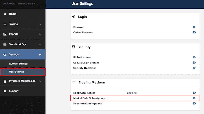
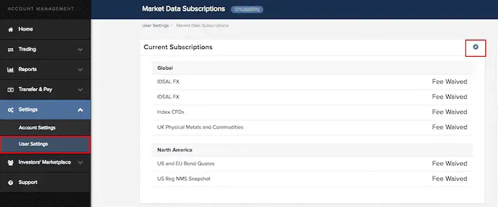
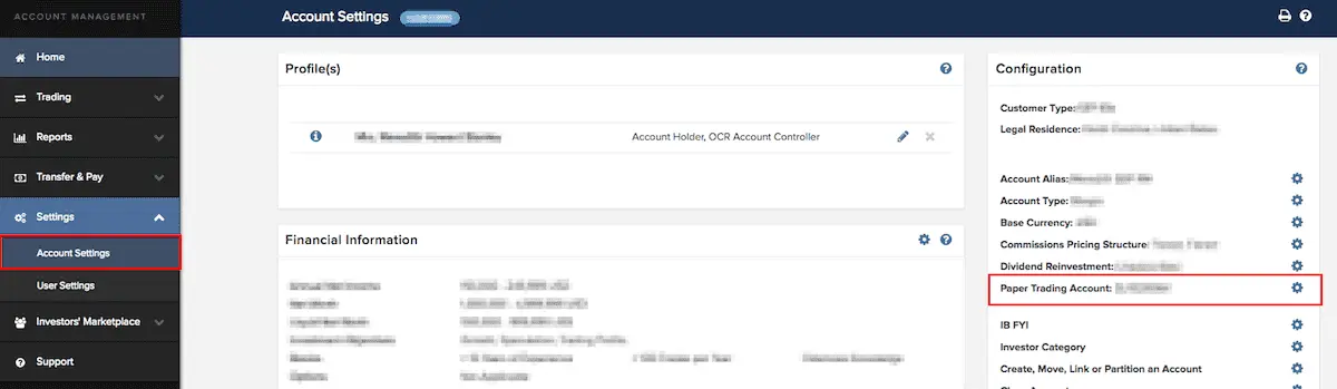
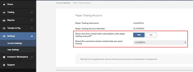
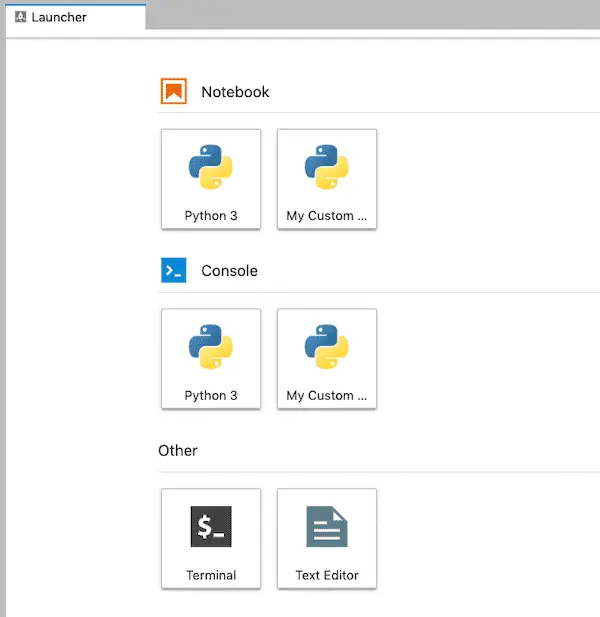
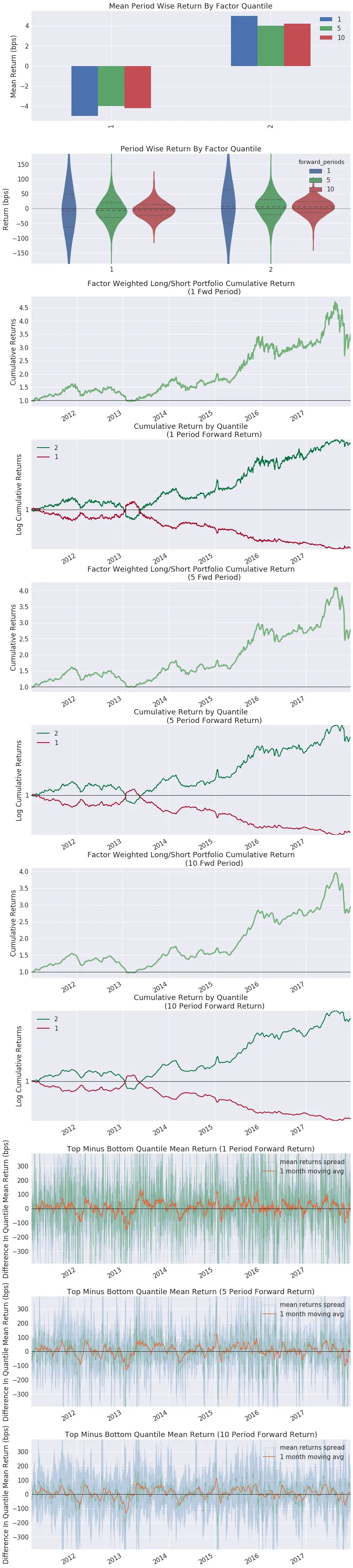
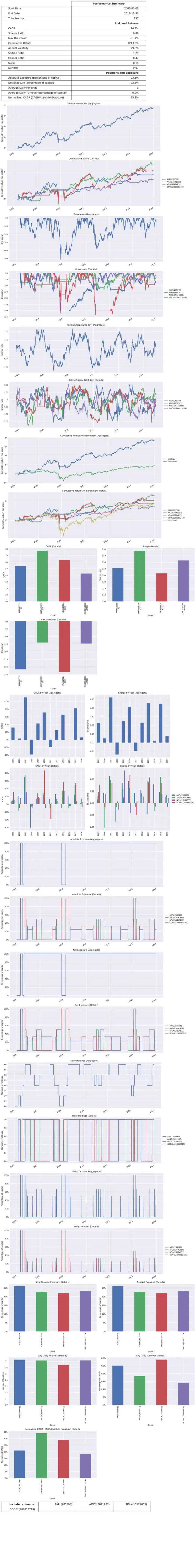
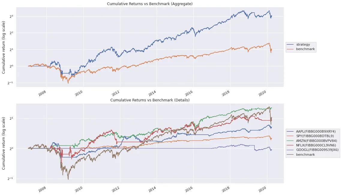
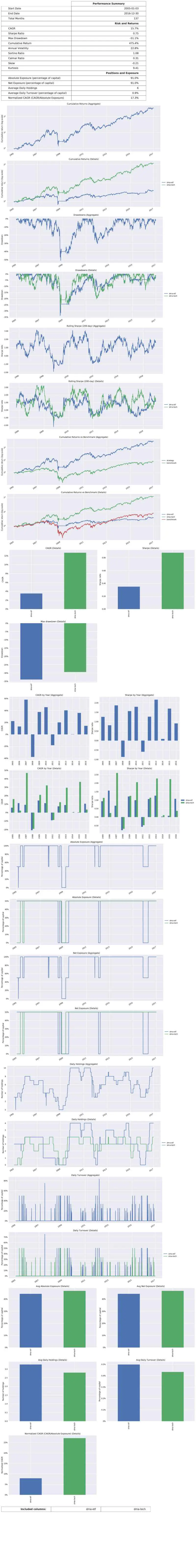
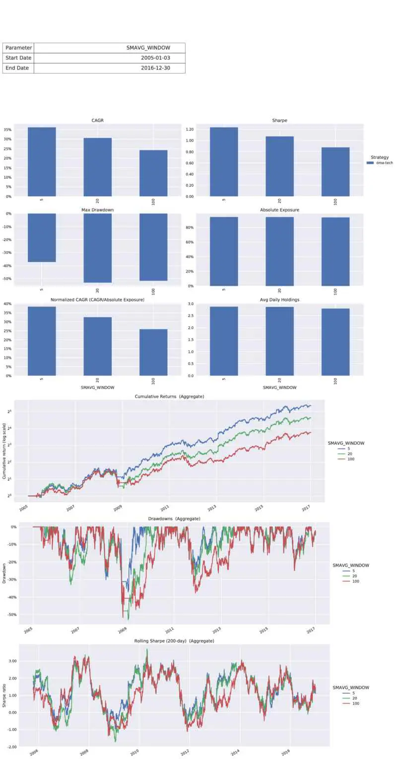
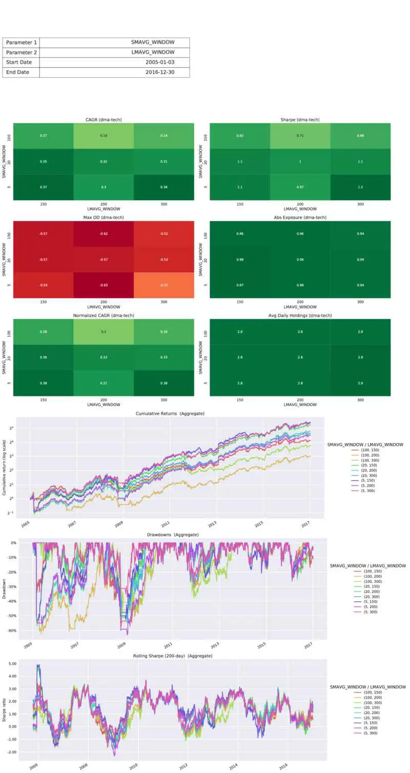
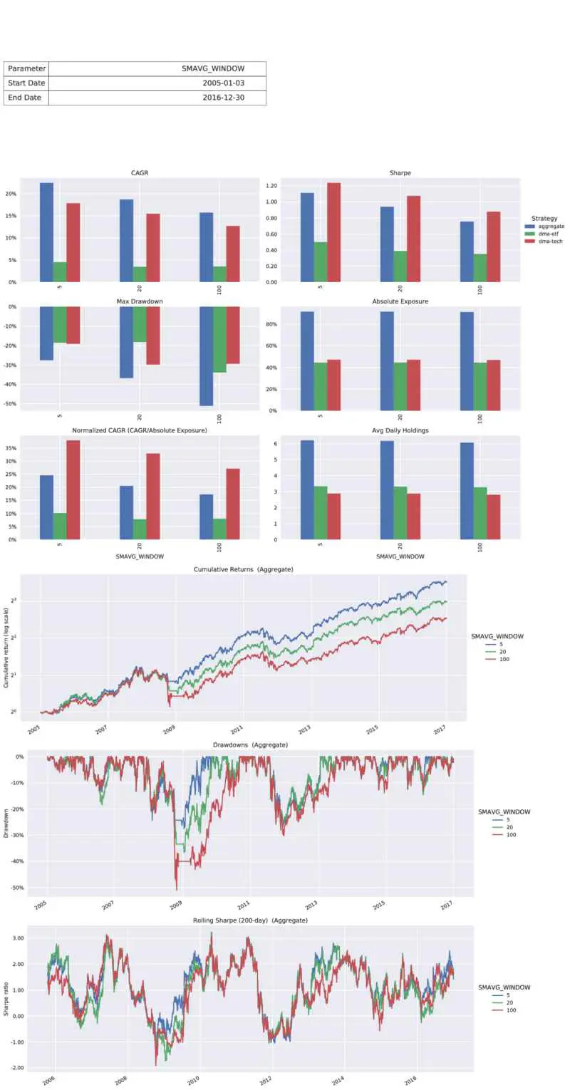
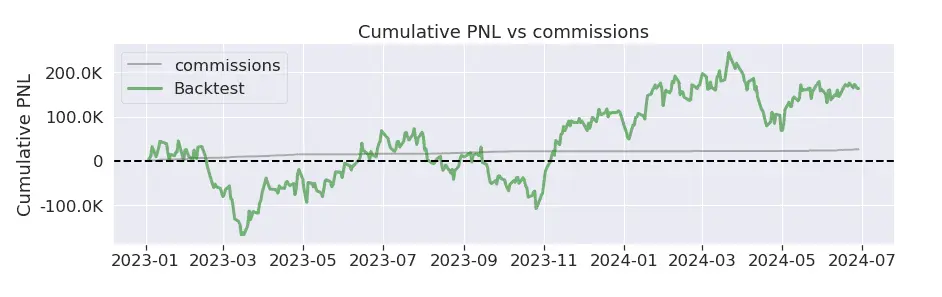
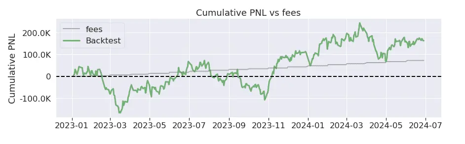

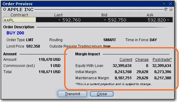

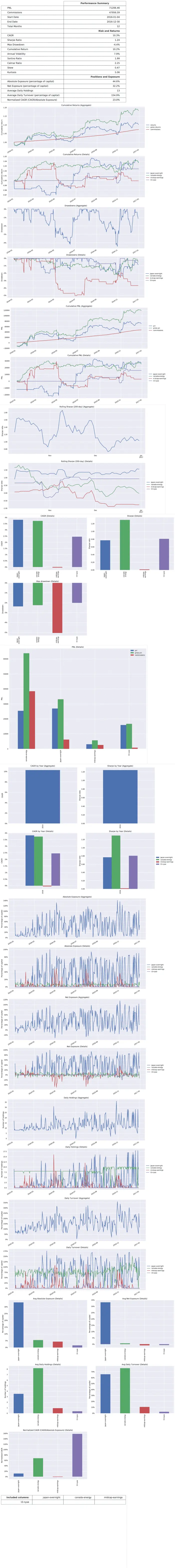
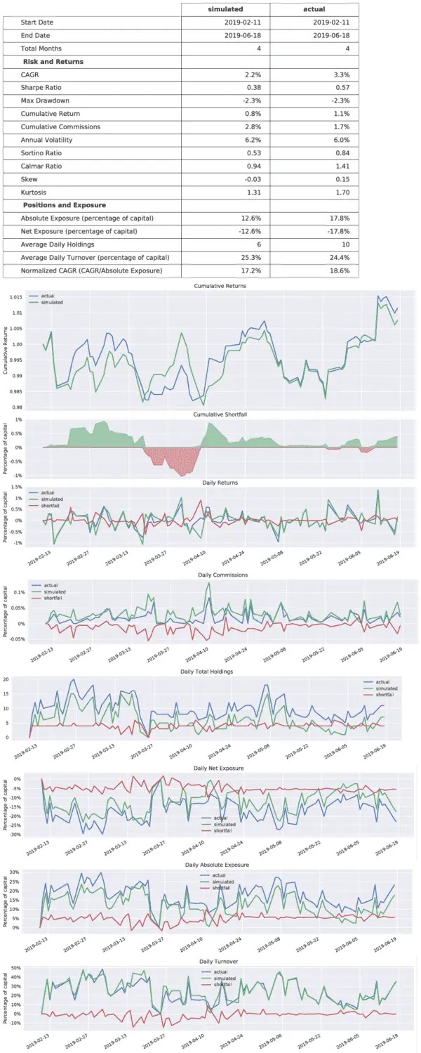
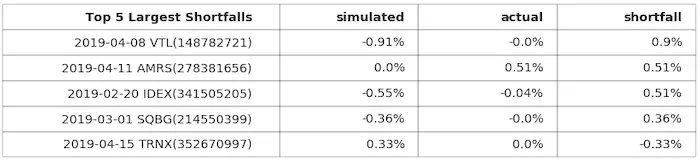

 Send a Message